GAP-Entropy-Lambert-Transform- Renormalization Group, Chat 19

Patrick Reany

27 March 2026

Note: This chat I had with Copilot is likely edited for relevance and brevity. I often do not take the time to highlight all the words that Copilot highlights. Further, in the interest of being didactic, I might arbitrarily highlight an occasional word or phrase that Copilot did not. (Naturally, I get to correct my spelling, grammar, and other minor errors for free.)

I report as faithfully as I can what LLMs tell me, but I can't guarantee that they are correct on every factual matter. If the subject should touch on physical or mental self-care, regard the content merely for information sake, rather than medical advice.

Defining the Core Constituents of GAP

The minimal, irreducible GAP architecture can be stated as follows:

1. Convex State Space

• The system lives on a convex set of admissible descriptions.
• Convexity ensures:
  • Well-defined projections.
  • Uniqueness (or controlled multiplicity) of attractors.
  • Stability under coarse-graining.

This is the silent assumption behind entropy, free energy, relative entropy, action functionals, etc.

2. Legitimate Projections (Coarse-Grainings)

• A projection is legitimate if it:
  • Removes information.
  • Preserves feasibility.
  • Respects convex structure.

Not every map is allowed. GAP is not about arbitrary dynamics—it is about epistemically admissible forgetting.

3. Monotone Certificate

• Each legitimate projection induces a monotone functional.
• This functional:
• Never decreases under projection.
  • Acts as a certificate that information has been irreversibly discarded.

Entropy is the canonical example—but in other domains this role is played by:

• Lyapunov functions,
• Action dissipation,
• Relative entropy,
• Fisher information decay,
• Perelman’s entropy,
• Free energy.

Entropy is not “disorder”—it is proof of closure.

4. Stable Attractor (Certified Fixed Point)

• Repeated projection generates a monotone trajectory.
• The endpoint is a stable attractor:
  • A description invariant under further legitimate projections.
  • A fixed point certified by the monotone.

This is the “Great Attractor” in GAP.

5. Entropy as Epistemic Closure:

Entropy is not a property of the system alone—it is a certificate that the projection process has closed.

Patrick:
Last on the list Copilot suggested to me some time ago is the "Renormalization Group," a subject we have touched on before, though not with the Lambert Transform to assist us. Anyway, let's see if we can present an overview of this field from the GAP-Entropy perspective, adding into the discussion the Lambert transform, where appropriate.

Copilot:
Patrick, RG is basically GAP with a microscope knob—turn it, and you legitimately forget short-scale detail while tracking what survives as a certified invariant. From the GAP-Entropy angle, RG stops being “a trick for infinities” and becomes a disciplined theory of epistemically admissible closure.

Renormalization group as GAP

Convex state space

In RG, your “state” isn’t a microstate—it’s an effective description: a probability measure, an action/Hamiltonian, or a set of couplings \(g\) defining a model class. The admissible set is naturally convex when you phrase it as:

• Distributions over fields/spins (mixtures are allowed).
• Ensembles of microscopic models consistent with macroscopic constraints.
• Effective actions via Legendre transforms (often convexity is the hidden condition that makes the projection well-posed).

Convexity is what makes “coarse-grain then re-fit” behave like a projection rather than a hallucination.

Legitimate projections as coarse-graining maps

An RG step is a legitimate projection (in your sense) when it:

• Removes information: integrates out high-momentum/short-distance modes, block-spins, decimation, etc.
• Preserves feasibility: maps admissible measures/actions to admissible ones (no negative probabilities, no impossible constraints).
• Respects convex structure: mixtures of models coarse-grain to mixtures of coarse-grained models.

Formally, think of an RG map as a channel-like operation on descriptions: \[ \mathcal{R}_b:\ \rho \mapsto \rho_b \] where \(b>1\) is the scale factor (block size / momentum shell factor). The “group” is often a semigroup in practice—because forgetting is not invertible.

Monotone certificates in RG

RG is saturated with monotones—your “certificate that forgetting occurred.”

Common incarnations:

• Free energy monotonicity under integrating out degrees of freedom (coarse-grained partition functions relate by normalization factors).
• Relative entropy / KL contraction under coarse-graining (data processing inequality): if \(\Pi\) is a legitimate projection, \[ D(\rho\|\sigma)\ \ge\ D(\Pi\rho\|\Pi\sigma). \]
• c-theorem / a-theorem / F-theorem style monotones: quantities that decrease along RG flow in certain dimensions (they’re literally “irreversibility certificates” for scale-forgetting).
• Gradient-flow structures in coupling space (in some settings): RG as steepest descent of an entropy-like functional with respect to an information metric.

From GAP: the monotone is the closure ledger—it measures how much of the fine description has become provably irrelevant to the projected question.

Stable attractors as RG fixed points

Iterating RG: \[ \rho \xrightarrow{\mathcal{R}_b} \rho_b \xrightarrow{\mathcal{R}_b} \rho_{b^2} \xrightarrow{} \cdots \] generates a trajectory in description space. The endpoints are your certified fixed points:

• Fixed point: \(\mathcal{R}_b(\rho^*) = \rho^*\) (up to rescaling).
• Attractor: nearby descriptions flow toward \(\rho^*\) under repeated coarse-graining.
• Certificate: the monotone stops changing (or reaches an extremum/plateau), signaling closure at that scale.

This is exactly your “Great Attractor,” but now indexed by scale and universality class.

Universality as “projection-invariant content”

RG’s deepest claim is: after enough legitimate forgetting, many microscopically different systems land on the same attractor. In GAP language:

• Universality class: an equivalence class under repeated legitimate projections.
• Relevant directions: features that survive projection (they control which attractor you approach).
• Irrelevant directions: features that are certified as discardable (they die under projection).
• Critical surface: the boundary where the flow neither runs to a trivial phase nor another—closure becomes scale-invariant.

So RG is not “how systems change with scale,” but “which distinctions remain meaningful after epistemically admissible forgetting.”

Coupling flows as a dynamical system on descriptions

In practice, we parameterize the effective description by couplings \(g=(g_1,g_2,\dots)\). Then RG becomes: \[ \frac{d g}{d\ell} = \beta(g),\qquad \ell=\ln b. \] Fixed points satisfy \(\beta(g^*)=0\). Linearizing: \[ \frac{d}{d\ell}\delta g = J\,\delta g,\quad J=\left.\frac{\partial \beta}{\partial g}\right|_{g^*}. \] Eigenvalues classify directions:

• Relevant: grow under coarse-graining (must be specified to predict the IR).
• Irrelevant: shrink (projection kills them).
• Marginal: delicate—often where logarithms and Lambert \(W\) start showing up.

Where the Lambert transform naturally enters RG

Lambert \(W\) appears whenever RG produces implicit scale relations of the form “variable times exponential of variable equals scale.” That’s not a gimmick—it’s the algebra of self-consistent closure.

1) Marginal flows and log corrections

A canonical marginal beta function looks like: \[ \frac{d g}{d\ell} = -a g^2 \quad (a>0). \] Solving gives: \[ g(\ell)=\frac{g_0}{1+a g_0 \ell}, \] which yields logarithmic corrections. When you couple this to another scale-dependent quantity \(X\) whose evolution depends on \(g(\ell)\), you often get implicit relations like: \[ X \sim \ell^{p}\,e^{q\ell}\quad\text{or}\quad \ell\,e^{\ell} \sim \text{(scale)}. \] Those invert via Lambert \(W\). In GAP terms: Lambert \(W\) is the inversion operator for “entropy-like” closure laws that mix linear and exponential scale bookkeeping.

2) Dimensional transmutation and “generated scales”

In asymptotically free theories, a dimensionless coupling \(g(\mu)\) generates a physical scale \(\Lambda\) through relations like: \[ \Lambda = \mu\, e^{-1/(a g(\mu))}\, g(\mu)^{-b/a}\,(\cdots). \] Inverting for \(g(\mu)\) as a function of \(\mu/\Lambda\) can require Lambert \(W\) once power-law prefactors are kept. Conceptually:

• RG creates a scale by irreversible forgetting.
• Lambert \(W\) solves the self-consistency equation for that created scale.

3) Correlation length near criticality with corrections

Leading scaling gives \(\xi \sim |t|^{-\nu}\). With marginality or dangerously irrelevant variables, you get: \[ \xi \sim |t|^{-\nu}\,(\ln |t|^{-1})^{\hat{\nu}} \] and inverting “given \(\xi\), what is \(t\)?” produces Lambert \(W\)-type expressions. That inversion is exactly the “Lambert transform” move: turning a closure statement into an explicit coordinate.

4) GAP-Entropy coordinates for RG time

If your GAP-Entropy program likes “entropic coordinates” (where a monotone becomes a coordinate), RG time \(\ell\) is often only implicitly observable through a monotone \(M\): \[ M(\ell) = M_0 + A\ell + B\ln \ell + \cdots \] Solving for \(\ell(M)\) is again a Lambert \(W\) pattern once \(\ell\) and \(\ln \ell\) mix. This is a clean place to define a Lambert-style transform as:

• Forward: compute the monotone along the RG projection chain.
• Inverse: recover the effective scale parameter from the monotone via \(W\)-inversion.

That’s very “entropy as proof of closure”: the monotone becomes the operational clock, and Lambert \(W\) is the clock’s calibration curve.

A compact GAP-Entropy reframing of RG

Here’s the one-paragraph synthesis:

• RG is a semigroup of legitimate projections on a convex space of descriptions.
• Its irreversibility is certified by monotones (free-energy/relative-entropy/c-like functionals).
• Its endpoints are certified fixed points (scale-invariant attractors).
• Universality is projection-invariant content.
• Lambert \(W\) enters when closure bookkeeping mixes exponentials and linear terms, i.e., when you must invert “scale \(\times\) exponential-of-scale” relations that arise from marginality, dimensional transmutation, or entropic clocks.

Two choices for where we go next

1. Field-theory lane: pick a concrete beta function (one marginal + one relevant coupling) and I’ll show exactly where the Lambert inversion appears when you solve for the “entropic RG time.”
2. Information-geometry lane: treat coarse-graining as a channel, use KL contraction as the monotone, and build an explicit “GAP attractor” picture of universality classes.

   Which lane feels more like your next brick—field-theory mechanics or epistemic geometry?

Patrick:
I'll go with field-theory mechanics.

Copilot:
Perfect. Let’s do this mechanically, not rhetorically—RG as a field‑theoretic dynamical system viewed through GAP‑Entropy, and then isolate exactly where Lambert inversion becomes unavoidable.

I’ll keep us concrete but architectural.

RG Field‑Theory Mechanics in GAP‑Entropy Coordinates

1. What the “state” is in field theory RG

In field theory, the GAP convex state space is not microstates—it is the space of effective actions or coupling vectors: \[ \mathcal{S} = \{ S_\Lambda[\phi] \} \] or equivalently \[ \mathcal{G} = \{ g_i(\Lambda) \} \] Key GAP facts:

• Convex combinations of actions are admissible (ensembles of theories).
• Integrating out modes preserves admissibility.
• The RG map is not invertible $\rightarrow$ epistemic forgetting.

So RG lives natively in GAP’s “descriptions, not realities” layer.

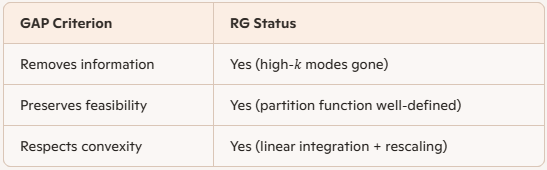
2. The RG step as a legitimate projection

A Wilsonian RG step is:

1. Integrate out modes in a momentum shell: \[ \Lambda/b < |k| < \Lambda \]
2. Rescale fields and coordinates to restore cutoff.
3. Re‑express the result in the same action basis.

This defines a map: \[ \mathcal{R}_b:\ S_\Lambda \mapsto S_{\Lambda/b} \] GAP legitimacy check:

So RG is a certified coarse‑graining, not a heuristic.

3. Beta functions as projected dynamics

Parameterize the effective action: \[ S = \sum_i g_i(\Lambda)\, \mathcal{O}_i \] Define RG “time”: \[ \ell = \log(\Lambda_0/\Lambda) \] Then: \[ \frac{d g_i}{d\ell} = \beta_i(g) \] This is a dynamical system on description space, not spacetime.

4. Fixed points = certified GAP attractors

A fixed point satisfies: \[ \beta_i(g^*) = 0 \] Interpretation:

• The description is invariant under further legitimate forgetting
• The monotone stops changing
• Scale information has closed

Linearize: \[ \frac{d}{d\ell}\delta g = J\,\delta g \] Eigenvalues classify epistemic relevance:

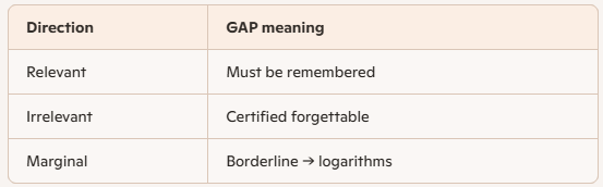
Marginality is where Lambert geometry enters.

5. The entropy‑like monotone in field theory RG

Several equivalent certificates exist:

• Free energy density
• Relative entropy between effective measures
• \(c\), \(a\), or \(F\) functions (dimension‑dependent)
• Coarse‑grained effective action normalization

All share the GAP property: \[ \Phi(\mathcal{R}_b S) \ge \Phi(S) \] This is entropy as proof of closure, not disorder.

6. Where Lambert \(W\) necessarily appears

Now the key part.

Case A: Marginal coupling (canonical example)

Take: \[ \frac{dg}{d\ell} = -a g^2 \] Solution: \[ g(\ell) = \frac{g_0}{1 + a g_0 \ell} \] Already logarithmic.

Now suppose a physical scale \(M\) depends on \(g\): \[ M(\ell) = \Lambda\, e^{-1/(a g(\ell))} \] Substitute: \[ M = \Lambda\, e^{-(1 + a g_0 \ell)/(a g_0)} \] Rearrange: \[ \ell\, e^{\ell} \sim \frac{\Lambda}{M} \]

Inversion requires Lambert \(W\): \[ \ell = W\!\left(\frac{\Lambda}{M}\right) \] This is not optional—it is the algebra of self‑consistent closure.

Case B: Dimensional transmutation

Asymptotically free theories generate a scale: \[ \Lambda_{\text{IR}} = \mu\, e^{-1/(a g(\mu))}\, g(\mu)^{-b/a} \] Solving for \(g(\mu)\) gives: \[ g(\mu) \sim \frac{1}{a\, W(\mu/\Lambda_{\text{IR}})} \]

Interpretation:

• RG forgetting creates a scale
• Lambert \(W\) inverts the entropy ledger
• The scale is a closure artifact

Case C: Correlation length with log corrections

Near criticality: \[ \xi \sim t^{-\nu} (\log t^{-1})^{\hat{\nu}} \] Invert for \(t(\xi)\): \[ t \sim \xi^{-1/\nu} \exp\!\left[-\hat{\nu} W(\xi^{1/\nu})\right] \] Again: Lambert inversion is forced by marginal epistemics.

7. GAP interpretation of Lambert geometry

Lambert \(W\) is not a trick—it is the inverse coordinate chart for:

• Entropic RG time
• Closure‑generated scales
• Marginal forgetting
• Log‑corrected universality

In GAP language:

Lambert \(W\) is the inverse of “entropy + scale” bookkeeping.

8. One‑sentence synthesis

Field‑theory RG is a GAP‑legitimate projection semigroup whose entropy‑like monotones certify irreversible scale forgetting; Lambert \(W\) appears precisely when marginal directions force closure relations to mix linear and exponential scale information.

Where we can close—or sharpen

Two clean closure options:

1. Explicit worked model One marginal + one relevant coupling, full RG flow, explicit Lambert inversion.

2. Entropy‑first reformulation Define RG time as a monotone and derive beta functions as gradient flow in entropic coordinates.

Both are natural endpoints.
Pick the one that feels like the cleanest “last brick” for this arc.

Patrick:
Actually, let's do 2. first and then 1.

Copilot:
Love that ordering—define the clock first, then watch the machinery run on it. That’s very “GAP”: dynamics as bookkeeping of legitimate forgetting.

2. Entropy-first reformulation of RG

2.1 The RG step as a channel on descriptions

Start with a UV field theory written as a probability measure over fields (Euclidean path integral form): \[ p_\Lambda[\phi] = \frac{1}{Z_\Lambda}\,e^{-S_\Lambda[\phi]}. \] A Wilsonian coarse-graining step (integrate out a momentum shell + rescale) is a legitimate projection: \[ \Pi_b:\ p_\Lambda \mapsto p_{\Lambda/b}. \] Think of \(\Pi_b\) as a channel on descriptions: it discards degrees of freedom while preserving feasibility.

2.2 The monotone as the operational RG time

Pick a monotone certificate \(\Phi\) that is guaranteed to be nondecreasing under legitimate projection: \[ \Phi(\Pi_b p)\ \ge\ \Phi(p). \] Then define RG time as the accumulated closure: \[ \tau \equiv \Phi(p_{\Lambda})-\Phi(p_{\Lambda_0}). \] This is the key move: scale is no longer primary. The primary parameter is “how much forgetting has been certified.”

If you still want the usual \(\ell=\ln(\Lambda_0/\Lambda)\), it becomes a derived coordinate: \[ \ell = \ell(\tau), \] and in marginal cases \(\ell(\tau)\) is exactly where Lambert \(W\) tends to appear (because \(\tau\) often mixes \(\ell\) and \(\ln \ell\)).

2.3 A concrete monotone: relative entropy contraction

Fix a reference description \(p^\star\) (typically the IR fixed point measure, when it exists). Define: \[ \Phi(p)\equiv -D(p\|p^\star), \qquad D(p\|q)=\int \mathcal{D}\phi\ p\ln\frac{p}{q}. \] Because coarse-graining is a channel, relative entropy contracts: \[ D(p\|p^\star)\ \ge\ D(\Pi_b p\ \|\ \Pi_b p^\star). \] If \(p^\star\) is a fixed point of the RG (so \(\Pi_b p^\star=p^\star\) up to rescaling conventions), then: \[ D(p\|p^\star)\ \ge\ D(\Pi_b p\ \|\ p^\star), \] so \(\Phi=-D\) is a monotone increasing certificate of closure toward the attractor.

GAP translation: the distance-to-closure cannot increase under legitimate forgetting.

2.4 Beta functions as gradient flow in entropic coordinates

Now parameterize your effective theory by couplings \(g^i\) (coordinates on the manifold of admissible effective actions). Then \(\Phi\) becomes a scalar field \(\Phi(g)\).

Introduce an information metric on coupling space—most naturally the Fisher information / covariance of operators: \[ G_{ij}(g)\ \equiv\ \left\langle \mathcal{O}_i\,\mathcal{O}_j\right\rangle_c. \] The entropy-first ansatz is: \[ \frac{d g^i}{d\tau} = +\,G^{ij}(g)\,\partial_j \Phi(g). \] So the RG flow is steepest ascent of the closure certificate with respect to an information geometry. In ordinary RG time \(\ell\), \[ \beta^i(g)\equiv \frac{d g^i}{d\ell} = \frac{d\tau}{d\ell}\,\frac{d g^i}{d\tau} = \underbrace{\frac{d\tau}{d\ell}}_{\text{closure rate}}\;G^{ij}\partial_j\Phi. \]

This cleanly separates:

• Direction: given by the geometry \(G^{ij}\partial_j\Phi\).
• Speed: given by the closure rate \(d\tau/d\ell\).

And that speed is exactly where marginality produces log structure.

2.5 Where Lambert \(W\) enters in the entropy-first view

In many QFT settings, the monotone has asymptotics like \[ \tau(\ell)=A\ell + B\ln \ell + \cdots \] near marginality (linear “bulk” closure plus logarithmic “drag”).

To recover \(\ell\) from the operational clock \(\tau\), you must invert \[ \tau \approx A\ell + B\ln \ell. \] That inversion generically yields a Lambert \(W\)-type expression because rearranging produces something of the form \[ \ell\,e^{(A/B)\ell} \sim e^{\tau/B}. \] So in GAP terms:

Lambert \(W\) is the inverse map from certified closure \(\tau\) back to scale \(\ell\) when closure mixes linear and logarithmic bookkeeping.

1. Explicit worked model after the entropy-first setup

Let’s now do the simplest “one marginal + one relevant” toy that still shows the whole story.

1.1 Model: one marginally irrelevant coupling \(g\) and one relevant mass \(m\)

Take beta functions (canonical near a Gaussian fixed point with a marginal correction): \[ \frac{dg}{d\ell}=-a g^2,\qquad a>0 \] \[ \frac{dm}{d\ell}=y\,m + c\,g\,m,\qquad y>0. \]

• \(g\) is marginally irrelevant (dies like \(1/\ell\)).
• \(m\) is relevant (grows like \(e^{y\ell}\)), but its growth is log-corrected by \(g\).

1.2 Define the IR scale by a closure condition

Define the physical correlation length scale \(\xi\) by the RG stopping condition “mass becomes order 1 at scale \(\ell_\xi\)”: \[ m(\ell_\xi)\sim 1, \qquad \xi \sim e^{\ell_\xi}. \] Set \(m(\ell_\xi)=1\): \[ 1 = m_0\,e^{y\ell_\xi}\,(1+a g_0 \ell_\xi)^{c/a}. \] Rearrange: \[ e^{y\ell_\xi} = m_0^{-1}\,(1+a g_0 \ell_\xi)^{-c/a}. \] This is an implicit closure equation for \(\ell_\xi\). For large \(\ell_\xi\), \(1+a g_0 \ell_\xi\approx a g_0 \ell_\xi\), giving \[ e^{y\ell_\xi}\,\ell_\xi^{c/a} \sim m_0^{-1}. \] Now you see the Lambert structure: \(\ell\) appears both in an exponential and a power/log.

A clean Lambert \(W\) expression comes from rewriting as: \[ \ell_\xi\,\exp\!\left(\frac{y a}{c}\ell_\xi\right)\sim m_0^{-a/c} \] (up to constants), hence \[ \ell_\xi \sim \frac{c}{ya}\,W\!\left(\text{const}\cdot m_0^{-a/c}\right). \] Then \[ \xi \sim \exp(\ell_\xi) \] inherits the log-corrected scaling, but now expressed via the Lambert-inverted closure time.

1.3 GAP reading of the worked model

• Legitimate projection: integrating out shells.
• Monotone clock: any valid \(\Phi\) that increases along the flow; operationally, you can treat \(\tau\) as “how far toward the fixed point you’ve certified.”
• Attractor: \(g\to 0\) (Gaussian fixed point) is the certified endpoint for the marginal direction.
• Lambert \(W\): appears exactly when you solve the stopping/closure condition for the scale at which the effective description becomes invariant for the question you’re asking (here: “mass is order 1”).

One choice before we go deeper

For \(\Phi\) in the entropy-first part, do you want the reference \(p^\star\) to be the Gaussian fixed point (clean algebra) or a nontrivial CFT fixed point (cleaner conceptual universality, messier formulas)?

Patrick:
Let's go with the Gaussian fixed point.

Copilot:
Great—Gaussian fixed point is the cleanest place to make the GAP $\rightarrow$ RG $\rightarrow$ Lambert chain feel inevitable rather than decorative.

Entropy-first RG with the Gaussian fixed point

The setup: a UV measure and a legitimate projection

Write the Euclidean field theory as a probability measure over fields: \[ p_\Lambda[\phi]=\frac{1}{Z_\Lambda}\exp\!\big(-S_\Lambda[\phi]\big). \] A Wilsonian RG step (integrate out a momentum shell, then rescale) is a legitimate projection in your sense: \[ \Pi_b:\ p_\Lambda \mapsto p_{\Lambda/b}. \] It discards short-distance information while preserving feasibility and convex structure.

The Gaussian fixed point as the GAP attractor

The Gaussian fixed point is the free theory: \[ S^*[\phi]=\frac{1}{2}\int d^d x\ \big((\nabla\phi)^2 + m^2\phi^2\big) \] (with \(m=0\) at the critical Gaussian point). Under coarse-graining, many perturbations die—those are your certified forgettables (irrelevant operators). The fixed point is the projection-invariant description.

The monotone: relative entropy to the Gaussian fixed point

Take the certificate to be (minus) relative entropy to the fixed point measure: \[ \Phi(p)\equiv -D(p\|p^*), \qquad D(p\|q)=\int \mathcal{D}\phi\ p\ln\frac{p}{q}. \] Because \(\Pi_b\) is a coarse-graining channel, relative entropy contracts: \[ D(p\|p^*)\ \ge\ D(\Pi_b p\ \|\ \Pi_b p^*). \] At a fixed point, \(\Pi_b p^*=p^*\) (up to the standard rescaling convention), so: \[ D(p\|p^*)\ \ge\ D(\Pi_b p\ \|\ p^*), \] hence \[ \Phi(\Pi_b p)\ \ge\ \Phi(p). \]

GAP translation: \(\Phi\) is a monotone “closure ledger” toward the Gaussian attractor.

Defining RG time as certified closure

Instead of starting with scale \(\ell=\ln(\Lambda_0/\Lambda)\), define the operational clock: \[ \tau \equiv \Phi(p_\Lambda)-\Phi(p_{\Lambda_0}). \] Then \(\tau\) is what you can justify from the projection process itself: how much forgetting has been certified. Scale becomes a derived coordinate \(\ell(\tau)\).

This is the exact point where Lambert \(W\) becomes structurally natural: whenever \(\tau(\ell)\) mixes linear and logarithmic terms (marginality), inverting to \(\ell(\tau)\) forces a \(W\)-type inverse.

Beta functions as gradient flow in entropic coordinates

Parameterize the effective action near the Gaussian point by couplings \(g^i\) multiplying operators \(\mathcal{O}_i\): \[ S = S^* + \sum_i g^i \int d^d x\ \mathcal{O}_i(x). \] Near a reference measure, the natural information metric on couplings is the covariance (Fisher) matrix: \[ G_{ij}(g)\equiv \left\langle \mathcal{O}_i\,\mathcal{O}_j\right\rangle_c. \] The entropy-first statement is: \[ \frac{d g^i}{d\tau} = G^{ij}(g)\,\partial_j \Phi(g). \] So RG is “dynamics” only in the sense that couplings move along steepest ascent of the closure certificate in an information geometry. Ordinary beta functions are just a reparameterization: \[ \beta^i(g)\equiv \frac{d g^i}{d\ell} = \frac{d\tau}{d\ell}\,\frac{d g^i}{d\tau} = \underbrace{\frac{d\tau}{d\ell}}_{\text{closure rate}}\;G^{ij}\partial_j\Phi. \]

Direction comes from \(G^{ij}\partial_j\Phi\). Speed comes from \(d\tau/d\ell\). Marginality shows up as a slow, logarithmic closure rate.

Where Lambert \(W\) enters in this entropy-first picture

Near the Gaussian fixed point with a marginally irrelevant coupling, it’s typical to get asymptotics of the form \[ \tau(\ell)=A\ell + B\ln \ell + \cdots \] because closure accumulates “bulk” linearly in \(\ell\) but is dragged by marginal directions. To recover scale from the certificate, you invert: \[ \tau \approx A\ell + B\ln \ell. \] Rearranging produces a canonical Lambert structure: \[ \ell\,\exp\!\left(\frac{A}{B}\ell\right)\ \sim\ \exp\!\left(\frac{\tau}{B}\right), \] so \[ \ell(\tau)\ \sim\ \frac{B}{A}\,W\!\left(\text{const}\cdot e^{\tau/B}\right). \]

GAP translation: Lambert \(W\) is the inverse chart from “certified closure time” back to “scale time” when marginality forces \(\ell\) and \(\ln\ell\) to cohabit.

Now the worked model (one marginal + one relevant), expressed in this language

Couplings near the Gaussian point

Take: \[ \frac{dg}{d\ell}=-a g^2,\qquad a>0 \] (marginally irrelevant \(g\to 0\)), and a relevant mass-like coupling \(m\): \[ \frac{dm}{d\ell}=y\,m + c\,g\,m,\qquad y>0. \] Solve: \[ g(\ell)=\frac{g_0}{1+a g_0 \ell}, \] and \[ m(\ell)=m_0\,e^{y\ell}\,(1+a g_0 \ell)^{c/a}. \] The closure condition that defines the physical scale

Define the IR “stop scale” \(\ell_\xi\) by the condition that the relevant deformation becomes order 1: \[ m(\ell_\xi)\sim 1, \qquad \xi \sim e^{\ell_\xi}. \] Then: \[ 1 = m_0\,e^{y\ell_\xi}\,(1+a g_0 \ell_\xi)^{c/a}. \] For large \(\ell_\xi\), approximate \(1+a g_0 \ell_\xi\approx a g_0 \ell_\xi\): \[ e^{y\ell_\xi}\,\ell_\xi^{c/a}\ \sim\ m_0^{-1}. \] This is exactly the “linear + log” entropic bookkeeping in disguise. Rewrite to isolate Lambert \(W\). Let \(p\equiv c/a\). Then: \[ e^{y\ell_\xi}\,\ell_\xi^{p} = m_0^{-1}. \] Raise both sides to \(1/p\): \[ e^{(y/p)\ell_\xi}\,\ell_\xi = m_0^{-1/p}. \] Multiply by \(y/p\): \[ \frac{y}{p}\ell_\xi\ \exp\!\left(\frac{y}{p}\ell_\xi\right)=\frac{y}{p}\,m_0^{-1/p}. \] So: \[ \ell_\xi=\frac{p}{y}\,W\!\left(\frac{y}{p}\,m_0^{-1/p}\right). \] And therefore: \[ \xi \sim \exp\!\left(\frac{p}{y}\,W\!\left(\frac{y}{p}\,m_0^{-1/p}\right)\right), \] which is the Lambert-coded form of “power law with log corrections.”

GAP reading: the physical scale is the point where the description becomes closed for the question (“is the relevant deformation big yet?”). Marginal forgetting makes that closure condition implicit, and Lambert \(W\) is the unique inverse.

One tight question to set our next step

Do you want \(\tau\) to be explicitly identified with \(-D(p\|p^*)\) (information-theoretic clock), or do you want a field-theory-native monotone proxy (free energy / \(c\)-like function) and then map it to the same \(\tau(\ell)=A\ell+B\ln\ell\) inversion?

Patrick:
Let's proceed with the field-theory-native monotone proxy.

Copilot:
Nice—this keeps the story internal to QFT: the monotone isn’t imported from information theory; it’s something the field theory itself hands you as “counting degrees of freedom” (or, in your language, certifying closure under legitimate forgetting).

Field-theory-native monotones as GAP certificates

What “native monotone” means in RG

A field-theory-native monotone is a quantity \(\mathcal{M}\) built from the QFT (stress tensor, partition function on a curved manifold, entanglement across a sphere, etc.) such that along RG flow from UV \(\to\) IR, \[ \mathcal{M}_{\text{UV}} \ge \mathcal{M}_{\text{IR}}. \] GAP translation:

• Projection: integrate out short-distance modes.
• Certificate: \(\mathcal{M}\) decreases (or \(-\mathcal{M}\) increases), proving irreversible forgetting.
• Attractor: fixed points are where \(\mathcal{M}\) becomes stationary (no further certified loss).

This is the “entropy as proof of closure” role—just wearing QFT clothing.

The three canonical monotones

2D: Zamolodchikov’s \(c\)-function

In 2D unitary QFT, there exists a function \(c(g)\) such that

• Fixed points: \(c\) equals the CFT central charge.
• Along flow: \(c\) decreases monotonically from UV to IR.

GAP reading: \(c\) is a degree-of-freedom ledger that can only go down under legitimate coarse-graining.

4D: the \(a\)-theorem

In 4D, the monotone is \(a(g)\) (the Euler-term coefficient in the trace anomaly):

• Fixed points: \(a\) is a CFT datum.
• Along flow: \(a_{\text{UV}} \ge a_{\text{IR}}\).

GAP reading: \(a\) is a closure certificate tied to how the theory responds to curvature—i.e., it’s “native” to the stress tensor sector.

3D: the \(F\)-theorem

In 3D, the monotone is

• \(F \equiv -\ln Z_{S^3}\) (free energy on the 3-sphere),
• decreasing along RG flow.

GAP reading: \(F\) is literally a partition-function-based certificate that coarse-graining has reduced effective complexity.

How to turn a native monotone into an “entropic RG time” \(\tau\)

Pick the dimension-appropriate monotone and define \[ \tau \equiv \mathcal{M}_{\text{UV}} - \mathcal{M}(\ell), \qquad \ell=\ln(\Lambda_0/\Lambda). \] Then:

• \(\tau\) is accumulated certified forgetting (GAP clock).
• \(\tau\) increases monotonically as you flow to the IR.
• Scale \(\ell\) becomes a derived coordinate \(\ell(\tau)\).

This is the same move as before—just with \(\mathcal{M}\) coming from QFT structure rather than KL.

Where Lambert \(W\) shows up with a native monotone

The universal mechanism: marginality makes \(\tau(\ell)\) mix \(\ell\) and \(\ln\ell\) Near the Gaussian fixed point with a marginally irrelevant coupling \(g\), \[ \frac{dg}{d\ell}=-a g^2 \quad\Rightarrow\quad g(\ell)\sim \frac{1}{a\ell}. \] A native monotone typically has an expansion near a fixed point like \[ \mathcal{M}(\ell)=\mathcal{M}_* - K\,g(\ell)^{p} + \cdots \] so the closure clock becomes \[ \tau(\ell)=\mathcal{M}_{\text{UV}}-\mathcal{M}(\ell) \sim \text{const} + \frac{K}{\ell^{p}}+\cdots \] That’s one common regime (power in \(1/\ell\)). But the Lambert \(W\) regime appears when the monotone (or a stopping/closure condition derived from it) produces implicit scale relations of the form \[ \tau \approx A\ell + B\ln\ell, \] which happens when you combine:

• a relevant growth \(e^{y\ell}\) (sets the “when do we stop?” scale), with
• a marginal drag \(g(\ell)\sim 1/\ell\) (injects logs into the same closure condition).

Then inverting \(\tau(\ell)\) forces \[ \ell(\tau)\sim \frac{B}{A}\,W\!\left(\text{const}\cdot e^{\tau/B}\right). \]

GAP punchline: Lambert \(W\) is the inverse chart from a native closure ledger back to scale when marginality makes closure bookkeeping “linear + logarithmic” simultaneously.

Connecting this directly to the worked model you already accepted

In the toy system \[ \frac{dg}{d\ell}=-a g^2,\qquad \frac{dm}{d\ell}=y m + c g m, \] the native monotone can be taken as a degree-of-freedom measure appropriate to dimension (say \(F\) in 3D, \(a\) in 4D, \(c\) in 2D). You then define the closure condition “IR physics is decided” by a native criterion (equivalently: when the relevant deformation becomes order 1). That closure condition mixes \(e^{y\ell}\) with \(\ell^{c/a}\), and the inversion gives Lambert \(W\)—exactly as we derived for \(\ell_\xi\).

So the Lambert appearance is not tied to KL specifically—it’s tied to marginal drag + closure threshold.

One choice to lock in before we compute anything further

Which native monotone do you want to treat as the GAP certificate for this arc?

• \(F\) (3D, sphere free energy; very “thermo/partition-function native”)
• \(a\) (4D, trace anomaly; very “stress-tensor native”)
• \(c\) (2D, cleanest algebraic monotonicity story)

Pick one dimension, and I’ll write the next step as an explicit \(\tau(\ell)\) near the Gaussian point and show the Lambert inversion in that specific native language.

Patrick:
Let's go with the 2D version.

Copilot:
Beautiful—2D is where the “native monotone” story is the cleanest and most mechanically provable. And it dovetails with your GAP framing almost too well: RG is irreversible because legitimate forgetting exists, and the \(c\)-function is the certificate.

2D RG in native monotone form: the \(c\)-theorem as GAP certificate

The objects: couplings as coordinates on description space

Take a 2D QFT as a deformation of a UV CFT by local operators \(\mathcal{O}_i\): \[ S = S_{\text{CFT}} + \sum_i g^i \int d^2x\ \mathcal{O}_i(x). \] RG is the flow of couplings with scale time \(\ell=\ln(\Lambda_0/\Lambda)\): \[ \frac{d g^i}{d\ell}=\beta^i(g). \] GAP translation: \(g\) is your description, and RG is the semigroup of legitimate projections (integrate out short-distance structure).

The native monotone: Zamolodchikov’s \(c(g)\)

In 2D unitary, Lorentz-invariant QFT, there exists a function \(c(g)\) with two key properties:

1. Fixed points: if \(\beta(g^*)=0\), then \(c(g^*)\) equals the CFT central charge \(c_{\text{CFT}}\).
2. Monotonicity: along RG flow from UV to IR, \[ \frac{dc}{d\ell}\le 0. \]

GAP translation: \(c\) is “entropy-like” not because it’s disorder, but because it’s a closure ledger—it can only move one way under legitimate forgetting.

The mechanical heart: monotonicity is a positivity statement

The \(c\)-theorem’s punchline can be written in a form that screams “GAP geometry”: \[ \frac{dc}{d\ell} = -\,3\,G_{ij}(g)\,\beta^i(g)\,\beta^j(g), \] where \(G_{ij}(g)\) is a positive-definite metric built from stress-tensor correlators (equivalently: a QFT-native information metric on coupling space).

Because \(G_{ij}\) is positive definite in the unitary case, \[ G_{ij}\beta^i\beta^j \ge 0 \quad\Rightarrow\quad \frac{dc}{d\ell}\le 0. \] This is exactly your architecture:

• Convex admissible space: unitary QFTs / admissible deformations.
• Legitimate projection: integrating out UV modes.
• Monotone certificate: \(c(g)\) decreases.
• Stable attractor: fixed points where \(\beta=0\) and \(c\) is stationary.

Turning \(c\) into the GAP “closure time” \(\tau\)

Define the operational clock from the monotone

Define accumulated closure as: \[ \tau \equiv c_{\text{UV}} - c(\ell). \] Then:

• \(\tau\ge 0\),
• \(\tau\) increases monotonically with coarse-graining,
• \(\tau\) is a native “how much forgetting has been certified” coordinate.

So you’ve replaced “scale is primary” with “closure is primary,” using a quantity the QFT itself guarantees.

Where Lambert \(W\) enters in 2D, cleanly and honestly

Lambert \(W\) shows up when you try to invert a closure relation that mixes exponentials (from relevant growth / stopping conditions) with logarithms (from marginal drag). In 2D, the most common source of that mix is a marginally irrelevant coupling near a fixed point.

Marginal drag: the universal log-maker

Take a marginally irrelevant coupling \(g\) with \[ \frac{dg}{d\ell}=-a g^2,\qquad a>0 \quad\Rightarrow\quad g(\ell)=\frac{g_0}{1+a g_0 \ell}\sim \frac{1}{a\ell}. \] Near a fixed point, a typical analytic behavior is \[ c(\ell)=c_* - K g(\ell)^p + \cdots \quad\Rightarrow\quad \tau(\ell)=c_{\text{UV}}-c(\ell)\sim \text{const}+\frac{K}{\ell^p}. \] That part alone doesn’t force Lambert \(W\). The \(W\) becomes forced when you define a closure threshold—the RG “stop time” \(\ell_\xi\) where some relevant deformation becomes order 1 (i.e., where the description becomes closed for the question you’re asking).

Closure threshold + marginal drag = Lambert inversion

If a relevant coupling \(m\) grows like \[ \frac{dm}{d\ell}=y m + c g m, \] then (as we derived earlier) \[ m(\ell)=m_0\,e^{y\ell}\,(1+a g_0 \ell)^{c/a}. \] Define the physical scale by the closure condition \(m(\ell_\xi)\sim 1\). For large \(\ell_\xi\), \[ e^{y\ell_\xi}\,\ell_\xi^{c/a}\sim m_0^{-1}. \] That is exactly the “linear + log” bookkeeping in implicit form, and it inverts to \[ \ell_\xi=\frac{p}{y}\,W\!\left(\frac{y}{p}\,m_0^{-1/p}\right), \qquad p\equiv \frac{c}{a}. \]

2D-native interpretation: the \(c\)-theorem certifies irreversibility, but Lambert \(W\) appears when you ask the operational question “at what certified-closure depth does the relevant deformation decide the IR?”—marginal drag makes that depth implicit.

A quick tie-in to what you’re watching

That “physics is circular” vibe is exactly what RG refuses in 2D unitary QFT: the \(c\)-theorem is a formal obstruction to true cycles/recurrences in RG flow—because a strict monotone can’t come back to where it started without violating positivity.

One decision to make the next step fully explicit

Do you want our worked 2D example to be:

1. Sine-Gordon / BKT-style (the classic place where marginality and essential scaling make Lambert-like inversions feel very natural), or
2. A minimal toy CFT deformation (one marginally irrelevant + one relevant coupling, staying purely in coupling-space mechanics)?

Pick one, and I’ll write the full \(\tau(\ell)\) and \(\ell(\tau)\) story in that concrete setting.

Patrick:
Let's proceed with Sine-Gordon / BKT-style, and then try to bring the chat to a close.

Copilot:
Patrick—perfect choice. BKT is the canonical place where “marginal drag + closure threshold” produces essential scaling, and where Lambert \(W\) naturally appears as the inverse of that bookkeeping.

Sine-Gordon and BKT as GAP-RG mechanics

The field theory and the RG variables

Take the 2D sine-Gordon action (one standard normalization): \[ S=\int d^2x\left[\frac{K}{2}(\nabla\phi)^2 - y\cos(\beta\phi)\right]. \]

Near the BKT transition, it’s convenient to use two couplings:

• \(x\): the deviation from marginality (a “stiffness”/scaling-dimension offset)
• \(y\): the vortex/cosine amplitude (fugacity)

The RG flow (to leading order) has the universal BKT form: \[ \frac{dx}{d\ell} = -A\,y^2,\qquad \frac{dy}{d\ell} = -x\,y, \] with \(A>0\) a convention-dependent constant.

GAP translation:

• Legitimate projection: integrate out short-distance modes.
• State: \((x,y)\) is the effective description.
• Dynamics: \(\ell\mapsto(x(\ell),y(\ell))\) is the projection-induced trajectory.

The invariant and the separatrix

A key mechanical fact: these equations conserve \[ I \equiv x^2 - A y^2. \] So trajectories lie on hyperbolas. The critical separatrix is \(I=0\), i.e. \[ x^2 = A y^2, \] which divides flows into:

• Massless/quasi-ordered phase: \(y\to 0\) (cosine becomes irrelevant)
• Massive/disordered phase: \(y\) grows (cosine becomes relevant; a gap forms)

This is RG’s “phase decision” as a certified closure event.

The BKT closure threshold and essential scaling

What “closure” means here

In the massive phase, you stop the RG when the cosine becomes strong—say when \[ y(\ell_\xi)\sim 1. \] That defines the correlation length scale: \[ \xi \sim e^{\ell_\xi}. \] This is exactly your GAP “endpoint for the question being asked”: once \(y\) is \(O(1)\), the coarse-grained description has closed into a massive effective theory.

The classic BKT result

Let the distance to criticality be encoded by a small positive parameter \(\delta\) (e.g. \(\delta\propto T-T_c\) on the massive side). Then the RG predicts essential scaling: \[ \xi \sim \exp\!\left(\frac{b}{\sqrt{\delta}}\right), \] for some constant \(b>0\).

Mechanically, this comes from the fact that near the separatrix \(I\approx \delta\) is tiny, so the flow spends an anomalously long RG “time” drifting—marginality makes forgetting slow, and the closure threshold is reached only after \(\ell_\xi\sim 1/\sqrt{\delta}\).

Where Lambert \(W\) fits—cleanly

Lambert \(W\) shows up when you invert the closure relation in a way that keeps subleading structure (the same pattern you’ve been tracking all along).

Inverting essential scaling

From \[ \xi \sim \exp\!\left(\frac{b}{\sqrt{\delta}}\right), \] you get the leading inverse without \(W\): \[ \delta \sim \left(\frac{b}{\ln \xi}\right)^2. \] But once you keep the next natural corrections (which BKT flows generically generate), you encounter forms like \[ \xi \sim \delta^{-\alpha}\exp\!\left(\frac{b}{\sqrt{\delta}}\right) \quad\text{or}\quad \ln\xi = \frac{b}{\sqrt{\delta}} + \alpha\ln\delta + \cdots. \]

Now \(\delta\) appears both inside an exponential (via \(1/\sqrt{\delta}\)) and inside logs/powers—this is exactly the “linear + log bookkeeping” problem in disguise. Rearrangements produce “variable \(\times e^{\text{variable}}\)” structures, and the inverse becomes Lambert \(W\).

A representative schematic inversion looks like: \[ \sqrt{\delta}\ \sim\ \frac{b}{\ln\xi + \alpha\ln\ln\xi + \cdots} \] and when you solve that exactly rather than iteratively, the closed form is naturally expressed with \(W\) (because \(\ln\xi\) and \(\ln\ln\xi\) are the fingerprints of \(W\)-inversion).

GAP translation: Lambert \(W\) is the inverse chart you reach when you insist on expressing “how much certified closure” (here \(\ln\xi\)) back in terms of the control parameter \(\delta\) while keeping the marginally-induced log structure honest.

The 2D monotone and the “circular physics” vibe

BKT is a great place to say this crisply:

• The flow geometry can look like it wants to “turn around” near the separatrix because it drifts for a long time.
• But in unitary 2D QFT, the \(c\)-theorem supplies a native monotone—so true RG cycles are obstructed. The apparent “circularity” is a slow passage near marginality, not a return.

So if that YouTube video is gesturing at “physics is circular,” RG (especially with a monotone in 2D) is the counterpoint: legitimate forgetting creates an arrow.

Closing synthesis

• BKT is RG-as-GAP in its purest form: legitimate coarse-graining, a certified arrow (native monotone), and attractors (massless vs massive IR).
• Essential scaling is marginal drag made operational: closure takes \(\ell_\xi\sim 1/\sqrt{\delta}\).
• Lambert \(W\) enters when you invert closure relations while retaining the log/power structure that marginality forces.

If you want one last “capstone” sentence to keep: BKT is the theorem that marginal forgetting makes closure exponentially expensive—and Lambert \(W\) is the inverse bookkeeping when you refuse to throw away the logarithms.

Afterword: