LaTeX graphics, Xy-Pic graphics

Patrick Reany

4/19/2023

For the time being, I want to show off just the basics of the Xy-pic package for typesetting
graphs and diagrams in a LaTeX document. We start by making sure that we have the commmand

\usepackage[all]{xy}

in the LaTeX document preamble. This program is commonly used to produce nice-looking line
graphics such as flow charts, block diagrams, and commutative diagrams (for category theory)
and similar mathematical flow diagrams, of which I'll demonstrate a few.

Feel free to use the code given below to use as is or to edit to get the diagram you need. And, of
course, you can find better tutorials elsewhere on the Internet. By the way, there is another similar
graphics program (LaTeX package) one can use, called TikZ, which I hope to write on someday.

I am about to show two diagrams, each made by a different version of the diagram tools that require
the packege \usepackage[all]{xy}. One is the environment \begin{xy}...\end{xy} and the other is
\xymatrix{....}. The latter is simpler to use, but is not setup to make complicated diagrams, which the
former is (at least this was BingChat's summation of their basic differences). So, I expect that most
of the diagrams I will show on this page will be formatted in the environment of \begin{xy}...\end{xy}.

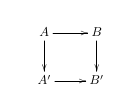
The following Xy-pic code will produce a so-called 'commutative diagram' with four corners, labeled
as: A at top left, B at top right, A' at bottom left, B' at bottom right:

\[
\xymatrix{
A \ar[r] \ar[d] & B \ar[d] \\
A' \ar[r] & B'
}
\]

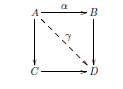
So, we redo it with a few small changes:

\begin{xy}
(0,20)*+{A}="a"; (20,20)*+{B}="b";%
(0,0)*+{C}="c"; (20,0)*+{D}="d";%
{\ar "a";"b"}?*!/_2mm/{\alpha};
{\ar "a";"c"};{\ar "b";"d"};%
{\ar "c";"d"};%
{\ar@{-->} "a";"d"};?*!/_2mm/{\gamma};
\end{xy}

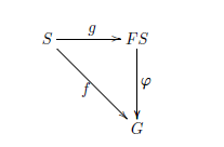
\begin{xy}
(0,20)*+{S}="a"; (20,20)*+{FS}="b";%
%(0,0)*+{C}="c";
(20,0)*+{G}="d";%
{\ar "a";"b"}?*!/_2mm/{g};
%{\ar "a";"c"};
{\ar "a";"d"}?*!/^2mm/{f};%
%{\ar "c";"d"};%
{\ar@{-->} "b";"d"};?*!/_2mm/{\varphi};
{\ar "b";"d"};?*!/_2mm/{\varphi};
\end{xy}

Notice that I have commented out the lines of code I didn't want to use in
this diagram, but might want to activate in a later version of the diagram.
In LaTeX, sometimes it's more efficient to comment out a line or lines of code
rather than the delete them.

\hskip1.6in
\hbox{$\displaystyle
\begin{xy}
(0,30)*+{\ket{\psi} \ket{0}}="a"; (40,30)*+{\ket{\psi} \ket{\psi}}="b";%
(0,0)*+{\alpha\ket{00} + \beta\thin \ket{10}}="c";%
(40,0)*+{\alpha\ket{00} + \beta\thin \ket{11}}="d";%
{\ar "a";"b"}?*!/_2mm/{U};%
{\ar "a";"c"}?*!/^2mm/{E}; % Added "E" label
{\ar "b";"d"}?*!/_2mm/{E};%
{\ar "c";"d"}?*!/^2mm/{U};%
%{\ar@{-->} "a";"d"}?*!/_2mm/{\gamma};
\end{xy}
$}

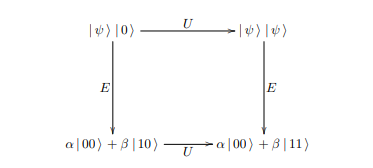
So, why did I put the xy diagram into an hbox? I did that so that I could control
the horizontal placement of the diagram. There could be a more elegant way to do
this. My problem is that I first coded in TeX back in the PlainTeX days, and this
is all I knew back then to do this kind of thing. The command \hskip1.6in shoves
the hbox and its contents 1.6 inches to the right.

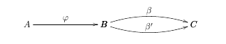
Epimorphism:

\hskip.75in\vbox{
\begin{xy}
{\ar@/^.75pc/(30,0)*+{B}; (65,0)*+{C}}%
?*!/_2mm/{\beta};%
{\ar@/_.75pc/(30,0)*+{B}; (65,0)*+{C}}%
?*!/_2mm/{\beta'};%
%{\ar@/_.75pc/(40,0)*+{B}; (70,0)*+{C}}%
%?*!/^2mm/{\varphi};%
{\ar (0,0)*+{A}; (30,0)*+{B}}%
?*!/_2mm/{\varphi};%
\end{xy}
}

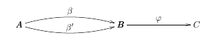
Monomorphism:

\hskip.75in\vbox{
\begin{xy}
{\ar@/^.75pc/(0,0)*+{A}; (40,0)*+{B}}%
?*!/_2mm/{\beta};%
{\ar@/_.75pc/(0,0)*+{A}; (40,0)*+{B}}%
?*!/_2mm/{\beta'};%
%{\ar@/_.75pc/(40,0)*+{B}; (70,0)*+{C}}%
%?*!/^2mm/{\varphi};%
{\ar (40,0)*+{B}; (70,0)*+{C}}%
?*!/_2mm/{\varphi};%
\end{xy}
}

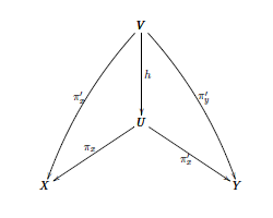
Cartesian Product One:

\hskip1.5in\vbox{
\begin{xy}
{\ar@/^.75pc/(30,50)*+{V}; (60,0)*+{Y}}%
?*!/_2mm/{\pi_y'};%
{\ar@/_.75pc/(30,50)*+{V}; (0,0)*+{X}}%
?*!/^2mm/{\pi_x'};%
{\ar (30,50)*+{V}; (30,20)*+{U}}%
?*!/_2mm/{h};%
{\ar (30,20)*+{U}; (0,0)*+{X}}%
?*!/^2mm/{\pi_x};%
{\ar (30,20)*+{U}; (60,0)*+{Y}}%
?*!/^2mm/{\pi_x'};%
\end{xy}
}

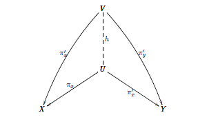
Cartesian Product Two:

\hskip1.5in\vbox{
\begin{xy}
{\ar@/^.75pc/(30,50)*+{V}; (60,0)*+{Y}}%
?*!/_2mm/{\pi_y'};%
{\ar@/_.75pc/(30,50)*+{V}; (0,0)*+{X}}%
?*!/^2mm/{\pi_x'};%
{\ar@{--} (30,50)*+{V}; (30,20)*+{U}}%
?*!/_2mm/{h};%
{\ar (30,20)*+{U}; (0,0)*+{X}}%
?*!/^2mm/{\pi_x};%
{\ar (30,20)*+{U}; (60,0)*+{Y}}%
?*!/^2mm/{\pi_x'};%
\end{xy}
}