Note: I'm using MathJax to code the mathematics in this webpage.
LaTeX matrices and determinants can be simple or complex, as we shall soon see. We won't do much with determinants because they're similar to matrices, yet usually simpler.
One usually thinks of a mathematical matrix as having 'sides', such as made with either a '['..']' pair or a '('..')' pair. But in LaTeX, our matrices come without those additions, apparently to give ease of defining them by the user or in certain packages. Array is the default in LaTeX and matrix is the default in amsmath. But there other differences, but in this introduction, I'll not go over them.
Note: \def\thinskip{\hskip.1in{}} is the definition for \thinskip.
The following code produces a beautiful table for displaying mathematics. The macro '\no' is short for \noindent.
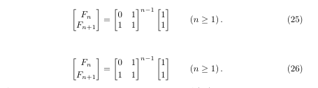
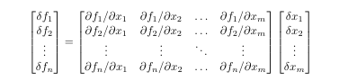
We start with three equations and their matrix representation. (Note: I dropped the \subequations commands because MathJax seemed to have trouble with them.)
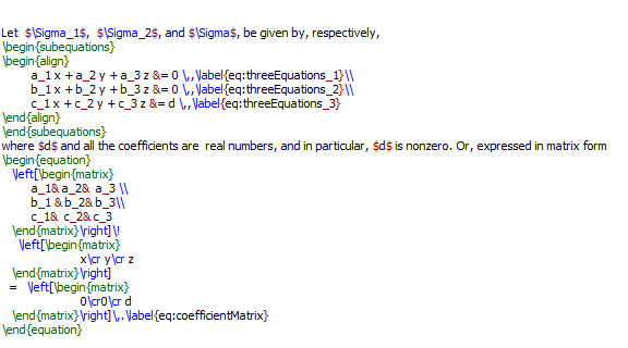
Let $\Sigma_1$, $\Sigma_2$, and $\Sigma$, be given by, respectively, \begin{align} a_1 x + a_2 y + a_3 z &= 0 \,,\label{eq:threeEquations_1}\\ b_1 x + b_2 y + b_3 z &= 0 \,,\label{eq:threeEquations_2}\\ c_1 x + c_2 y + c_3 z &= d \,,\label{eq:threeEquations_3} \end{align} where $d$ and all the coefficients are real numbers, and in particular, $d$ is nonzero. Or, expressed in matrix form \begin{equation} \left[\begin{matrix} a_1& a_2& a_3 \\ b_1 & b_2& b_3\\ c_1& c_2& c_3 \end{matrix}\right]\! \left[\begin{matrix} x\cr y\cr z \end{matrix}\right] = \left[\begin{matrix} 0\cr0\cr d \end{matrix}\right]\,.\label{eq:coefficientMatrix} \end{equation}
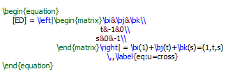
\begin{equation} [ED] = \left|\begin{matrix}\bi&\bj&\bk\\ t&-1&0\\ s&0&-1\\ \end{matrix}\right| = \bi(1)+\bj(t)+\bk(s)=(1,t,s) \,,\label{eq:u=cross} \end{equation}
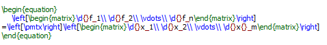
The point of this section is to show how to place a 'vector' matrix in the text.
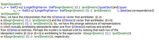
\begin{equation} u_+ = \half(1+u) \Longleftrightarrow \half\begin{bmatrix} 1\\ 1 \end{bmatrix}\quad\text{and}\quad u_- = \half(1-u) \Longleftrightarrow \half\begin{bmatrix} 1\\ -1 \end{bmatrix} \,.\label{eq:correspondence2} \end{equation} Now, we have the interpretation that the $2\times1$ vector that annihilates $I-J$ is $\begin{bmatrix} 1\\ 1 \end{bmatrix}$ and the $2\times1$ vector that annihilates $I+J$ is $\begin{bmatrix} 1\\ -1 \end{bmatrix}$. So, we have this strange admixture of representations in which mutually annihilating idempotents taken one from $2\times2$ matrices and another from $2\times1$ matrices. Perhaps the mystery is resolved a bit by noticing that each row of the idempotent matrix $I-J$ or $I+J$ is annihilating to the eigenvector $\begin{bmatrix} 1\\ 1 \end{bmatrix}$ or $\begin{bmatrix} 1\\ -1 \end{bmatrix}$, respectively.
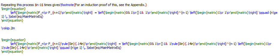
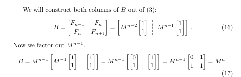
The only difference between the coding of the two lines is that in the second one, the command '\rule{0in}{.14in}'
was added to give a little more room between the rows. I couldn't use MathJax this time because, apparently, it doesn't
like that additional code.
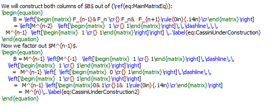
Where the code to make the vertical dashed line is
%to make vertical dashed lines
\makeatletter
\newcommand*\dashline{\rotatebox[origin=c]{90}{$\dabar@\dabar@\dabar@\dabar@\dabar@$}}
\makeatother
Postscript on this: I was not smart enough to figure out how to make this matrix with the dashed vertical
line in it, so I went on-line to find the answer. There are only four ways to get good at solving your
difficult LaTeX problem:
- Take a year out of your life to become an expert at it.
- Ask the guy across the hall from you is an expert at it and he doesn't mind you asking him questions.
- Do an Internet search on the topic. You might get lucky. I have found that if I can query with the
right search string and cut through the 'noise', I can get the answer I want. - I have had some luck asking ChatGPT and BingChat for assistance in this areas, but the real difficulty
here is being able to convey to the chatbot exactly what you want.
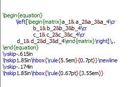
Or, patiently tweak out a solution. The following is a partition of a 4 X 4 matrix by two inner lines,
marking off the lower right submatrix.
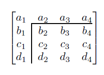
The following is the LaTeX code I used to produce it:
The explanation: First, make the matrix. Then, outside of the equation environment, create the first
line segment, either the horizontal one or the vertical one. You make it with the help of the \rule
command, which lets us create a rectangle of arbitrary width and length. A thin rectangle can pass
as a line segment, which is exactly what we want. The \rule command lets us make both vertical and
horizontal line segments. After we make one, we then have to move it into position into the matrix by
using a set of trial-and-error adjustments (with \hskip and \vskip) until it's just where we want it.
Then, be sure to use the \newline command to keep the second line segment placement independent
of the first.
You could even use this trick to create a Jordan Canonical form (Jordan Normal form) matrix, but
it would be a lot of work.
By the way, you can change the line separation inside a matrix with the \arraystretch command.

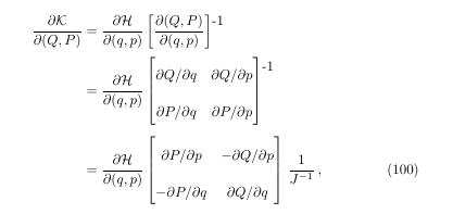
The point of this particular example is to show how to raise or lower an exponent to a matrix
(or determinant), which is what the '\raisebox' is for. (Undoubtedly there are other ways to do this.)
It seems that I didn't care for the default position LaTeX put it in.
Next,
with user-defined macros
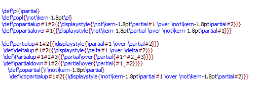
to produce the output
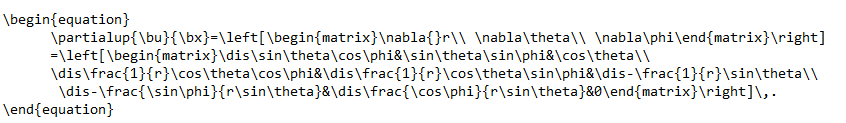
Notice that I have included the command '\dis' so that the fractions will be rendered in displaystyle.
\begin{equation} \partialup{\bu}{\bx}=\left[\begin{matrix}\nabla{}r\\ \nabla\theta\\ \nabla\phi\end{matrix}\right] =\left[\begin{matrix}\dis\sin\theta\cos\phi&\sin\theta\sin\phi&\cos\theta\\ \dis\frac{1}{r}\cos\theta\cos\phi&\dis\frac{1}{r}\cos\theta\sin\phi&\dis-\frac{1}{r}\sin\theta\\ \dis-\frac{\sin\phi}{r\sin\theta}&\dis\frac{\cos\phi}{r\sin\theta}&0\end{matrix}\right]\,. \end{equation}
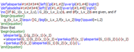
\no{}If $G_1(x_1,x_2,y),\ G_2(x_1,x_2,y)$, and $f(x_1,x_2)$ are given, and if \begin{equation} g_i(x_1,x_2)\equiv{}G_i\bigl(x_1,x_2,f(x_1,x_2)\bigr)\qquad(i=1,2) \end{equation} Show that \begin{equation} \abspartial{g_1}{g_2}{x_1}{x_2} =\abspartial{G_1}{G_2}{x_1}{x_2}+\partialup{f}{x_1}\abspartial{G_1}{G_2}{y}{x_2} +\partialup{f}{x_2}\abspartial{G_1}{G_2}{x_1}{y}\,. \end{equation}
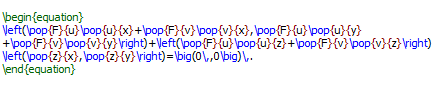
You can get the macro definitions for this code in the HTML file for this webpage.
\begin{equation} \left(\pop{F}{u},\pop{F}{v}\right)\left[\,\pmtwoXtwo{\dispop{u}{x}}{\dispop{u}{y}}{\dispop{v}{x}}{\dispop{v}{y}} +\pmtwoXone{\dispop{u}{z}}{\dispop{v}{z}}\left(\pop{z}{x},\pop{z}{y}\right)\,\right]=\big(0\,,0\big)\,. \end{equation}
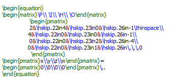
\begin{equation} \begin{matrix}\P\\ \I\\ \H\\ \O\end{matrix} \begin{pmatrix} 2&\hskip.22in4&\hskip.23in0&\hskip.26in-1\thinspace\\ 4&\hskip.22in0&\hskip.23in0&\hskip.26in-1\\ 0&\hskip.22in0&\hskip.23in2&\hskip.26in-4\\ 0&\hskip.22in0&\hskip.23in1&\hskip.26in\,\,\,0 \end{pmatrix} \begin{pmatrix}x\\y\\z\\w\end{pmatrix}= \begin{pmatrix}0\\0\\0\\0\end{pmatrix}\,.%\eqno(44) \end{equation}
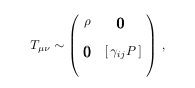
This next example is a hack, but I don't yet know a better way to do this:
The LaTeX code for this is
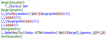
So, to construct this, I first made the parenthesis matrix with the pmatrix command.
I had to move the bold zeros to look good. Then I created the part about the [gamma
sub i,j P] and then moved it, by trial and error, until it fit into the pmatrix at
just the right spot. The '\,' command moves to the right a little, and the '\!' command
moves to the left a little.