The code for this is:
The code for this is:
\newcommand{\dothatr}{\skew1\dot{\hat r}}The \skew command lets us shove the overdot to the right.\begin{equation}
\dothatr = \frac{d}{dt} \hat r\,.
\end{equation}
Next
The code to this is:
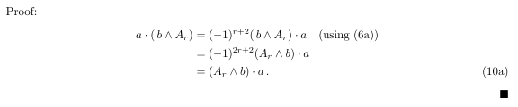
Proof:
\begin{subequations}
\begin{align}
a\cdot(\,b \wedge A_r) &=(-1)^{r+2}(\,b\wedge A_r)\cdot a\quad\text{(using (\ref{eq:ThirdEq.a}))} \notag\\
&=(-1)^{2r+2}(A_r\wedge b)\cdot a \notag\\
&= (A_r\wedge b)\cdot a \,.
\end{align}
\end{subequations}
\hfill$\blacksquare$
\vskip.15in
Next
The code to this is:
\begin{equation}where I defined \hba as
A_\pm = \alpha(1 \pm \hba) \,.\label{eq:A.idempotent}
\end{equation}
\newcommand{\hba}{\hat\ba}
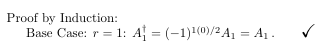
\no Proof by Induction:
Base Case: $r=1$: $ A_1^\dagger = (-1)^{1(0)/2} A_1 = A_1\,.\qquad \mathlarger{\mathlarger{\mathlarger{\checkmark}}}$
The \usepackage{relsize} package gives options to make a math symbol larger or smaller (\mathsmaller), and, as you can see, it can be nested. To get the checkmark symbol, use the package \usepackage{amssymb}.
Next,
The code to this is:
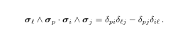
\begin{equation}I used the definition: \newcommand{\bsigma}{\boldsymbol{\sigma}} to make a bold version of the sigma, where \boldsymbol can use amsmath. A LaTeX advisory said that the package \usepackage{bm} will also work with the command '\bm', though I haven't tried this yet myself.
\bsigma_\ell\wedge\bsigma_p\cdot \bsigma_i\wedge\bsigma_j =
\delta_{pi} \delta_{\ell j} - \delta_{pj} \delta_{i\ell}\,.\label{eq:deltas}
\end{equation}
First note: Getting a bold version of a math symbol is confusing. For example, you can use
Second note: \boldsymbol is recognized in Mathjax, which is useful to know when putting LaTeX into HTML.
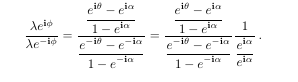
The code to this is:
\begin{equation}
\frac{\lambda e^{\bi\phi}}{\lambda e^{-\bi\phi}}
= \frac{\dis \frac{e^{\bi\theta}-e^{\bi\alpha}}{\dis1-e^{\bi\alpha}}}{\dis\frac{e^{-\bi\theta}-e^{-\bi\alpha}}{\dis1-e^{-\bi\alpha}}}
= \frac{\dis \frac{e^{\bi\theta}-e^{\bi\alpha}}{\dis1-e^{\bi\alpha}}}{\dis\frac{e^{-\bi\theta}-e^{-\bi\alpha}}{\dis1-e^{-\bi\alpha}}}
\frac{1}{\dis\frac{e^{\bi\alpha}}{e^{\bi\alpha}}} \,.\label{eq:Identity1.2}
\end{equation}
So, the point of this graphic is to show how to do nested fractions.
Next,
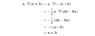
The code to this is:
\begin{align}
\ba\cdot\del (\bx\cross \bb)&= \ba\cdot\del (-i\bx\wedge \bb)\notag\\
&= -\frac{i}{2}\,\ba\cdot\del (\bx\bb - \bb\bx)\notag\\
&= -\frac{i}{2}\,(\ba\bb - \bb\ba)\notag\\
&= -i\,(\ba\wedge\bb)\notag\\
&= \ba\cross\bb\,.
\end{align}
where the bold symbols are user-defined. such as for \ba: \newcommand{\ba}{{\bf a}}.
Next,
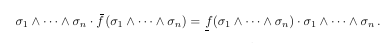
The code to this is:
\begin{equation}
\sigma_1\wedge\cdots\wedge \sigma_n \cdot \obf( \sigma_1\wedge\cdots\wedge \sigma_n)
= \ubf( \sigma_1\wedge\cdots \wedge\sigma_n) \cdot \sigma_1\wedge\cdots\wedge \sigma_n \,.
\end{equation}
I think that the simple '\overline f' and '\underline f' don't look good. This is just my personal feeling. So
I made a macro to make them look better:
\newcommand{\ubf}{\kern1pt{}f\kern-6pt\underline{\phantom{\lower2pt\hbox{i}}}\kern3pt{}}
\newcommand{\obf}{f\kern-3.2pt\skew1\overline{\phantom{l}}\kern1pt{}}
The code to this is:
Let $\bX = \Exterior_{i=1}^k \bx_i$.

The code to this is:
Let the set of vectors $\{\ba_1,\ba_2,\ldots,\ba_n\}$ be linearly independentwhere \definedas comes from \newcommand{\definedas}{\equiv}.
over an $n$-dimensional space, so that
\begin{equation}
A_n \definedas \ba_1\wedge\cdots\wedge \ba_n \ne0\,,
\end{equation}
The point is to first showcase both \ldots and \cdots, and then to explain when they're used. The ldots (dots on the line) mean that you've dropped an arbitrary number of serial items, typically separated by commas. The cdots (dots in the center of the line) mean that you've dropped an arbitrary number of serial items, typically connected by identical associative binary operators, such as '+' sign or, in this case, the wedge product.
Next,
The code to this is:
\begin{equation}
\pm L = \left(\frac{\gamma+1}{2}\right)^{1/2}\! + \, \hat\bv\left(\frac{\gamma-1}{2}\right)^{1/2}\,.\label{eq:pmL}
\end{equation}
![]()
The code to this is:
\begin{equation}
\bv_1 = \bv_1^\parallel + \bv_1^\perp\,,\label{eq:v_1breakup}
\end{equation}
The code to this is:
\begin{equation}
$\bigtriangleup (t_1\boldzero t') \sim \bigtriangleup (t'\boldzero t_2)$
\end{equation}
where I used: \newcommand{\boldzero}{\boldsymbol{0}}.
The code to this is:
\begin{equation}where I used the macro \newcommand{\select}[1]{\langle\, #1 \,\rangle}.
\select{\Omega_+V}_{0+1} = \select{\Omega_+V}_{0+1}^\dagger = \select{V\Omega_+^\dagger}_{0+1}\,,
\end{equation}
Next,
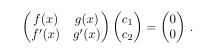
The code to this is:
\begin{equation}
\begin{pmatrix}f(x) & g(x) \\ f'(x) & g'(x)\end{pmatrix} \begin{pmatrix}c_1\\c_2\end{pmatrix}
= \begin{pmatrix}0\\0\end{pmatrix}\,.\label{MatrixEq.Appendix0}
\end{equation}
Next,
![]()
The code to this is:
\begin{equation}
\Perm{14}{3} = \binom{14}{3}\,3!\,.\label{eq:BinomFromPerm1}
\end{equation}
Next,
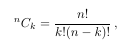
The code to this is:
\begin{equation}
\Comb{n}{k}=\frac{n!}{k!(n-k)!}\,,\label{eq:CombinationsFaction}
\end{equation}
Next, I encountered a problem with a matrix in an exponent -- it's too large!
Not to mention that the fraction is too small. The second figure is my solution
to this problem
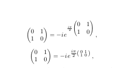
The code to this is in two parts: the first (naive) part that doesn't quite work,
and the second part that looks much better --- at least to me. By the way, the
command '\thin' I defined for myself; its purpose here is to insert a little extra
space for aesthetic reasons. Truth be told, I do a lot of tweaking for aesthetic
purposes.
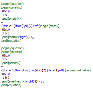
The solution to the matrix resizing turned out to be the special matrix environment
smallmatrix, which requires the [amsmath] package. By placing the smallmatrix
inside an hbox, I wanted to create an environment independent of the environment
outside of the hbox. (Perhaps another choice would be to use mbox.) The thing to
remember is that inside an hbox the natural environment is text, so one has to put
in the dollar signs to change it to inline math mode. Before I used smallmatrix, I
tried the usual modifiers like \small and \scriptstyle, but they did not work for me.