The code for this is:
The code for this is:
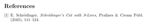
\begin{thebibliography}{9}The point of this obscure demonstration is because in some circumstances
\bibitem{Schrodinger} E.\ Schr\umlaut{o}dinger, {\it Schr\"odinger's Cat
with 9-Lives}, Pralines \& Cream Publ. (2165), 111--124.
\end{thebibliography}
\newcommand{\umlaut}[1]{{$\ddot{\hbox{#1}}$}}.
Others recommend that one use the package
\usepackage[utf8]{inputenc}
Next,
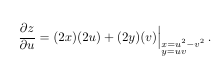
The code to this is:
\begin{equation}
\frac{\partial z}{\partial u}= (2x)(2u) + (2y)(v)\Big|_{\substack{x=u^2-v^2\\ y=uv\hfill}}\,.
\end{equation}
Next,
The code to this is:
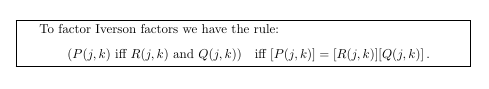
$$This code definitely goes back to my Plain TeX days. Alternatively, with
\boxed{\vbox{To factor Iverson factors we have the rule:
\vskip.1in
\hskip.3in($P(j,k)$ iff $R(j,k)$ and $Q(j,k)$)\quad iff $[P(j,k)] =[R(j,k)][Q(j,k)]$\,.
}}$$
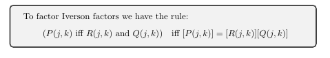
\usepackage{tcolorbox}
in the preamble, we can use
\begin{tcolorbox}
To factor Iverson factors we have the rule:
\vskip.1in
\hskip.3in($P(j,k)$ iff $R(j,k)$ and $Q(j,k)$)\quad iff $[P(j,k)] =[R(j,k)][Q(j,k)]$
\end{tcolorbox}
to get
Next,
![]()
The code to this is:
\begin{equation}
\text{Hom}(V,W)^* \definedas \{ \text{Hom}(V,W), \oplus, \cdot\}\,,\label{eq:Defn.Hom(V,W)^*}
\end{equation}
Notice that one can use a lot of non-alphanumeric symbols in a \label{} macro, but don't put a blackslash in it.
Next,
The code to this is:
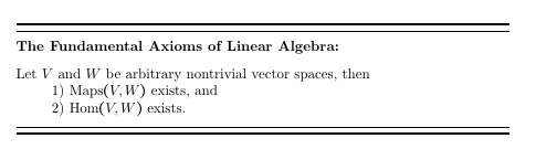
\no\rule{\textwidth}{1.2pt}
\vskip.05in
\hrule
\vskip.1in
\no{\bf The Fundamental Axioms of Linear Algebra:}
\vskip.1in
\no Let $V$ and $W$ be arbitrary nontrivial vector spaces, then \par
\hskip10pt 1) Maps$(V,W)$ exists, and\par
\hskip10pt 2) Hom$(V,W)$ exists.
\vskip.1in
\hrule
\vskip.05in
\no\rule{\textwidth}{1.2pt}
This code is basically just Plain TeX.
Next,
The code to this is:
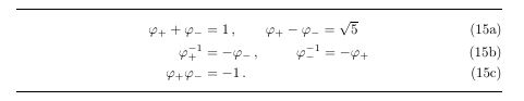
\vskip.15in
\hrule
\begin{subequations}
\begin{align}
\varphi_{+} +\varphi_{-} &= 1\,, \qquad \varphi_{+} -\varphi_{-} = \sqrt{5}\\
\varphi_{+}^{-1} &= -\varphi_{-}\,,\qquad\hskip.08in \varphi_{-}^{-1} = -\varphi_{+}\label{eq:PhiInverses}\\
\varphi_{+} \varphi_{-} &= -1 \,.
\end{align}
\end{subequations}
\hrule
\vskip.15in
So, the point of this graphic is to demonstrate alignment.
Next,
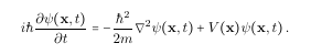
The code to this is:
\begin{equation}
i\hbar \partialup{\psi(\bx,t)}{t} = - \frac{\hbar^2}{2m} \del^2 \psi(\bx,t) + V(\bx) \psi(\bx,t)\,.\label{eq:SchrodingerEq}
\end{equation}
The time-dependent Schrödinger Equation. (To get the o umlaut in HTML,
you have to use a special character string.)
Next,

The code to this is:
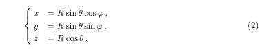
\begin{equation}
\left.\begin{matrix}x=r\sin \theta \cos \phi\\
y=r\sin\theta\sin\phi\\
z=r\cos\theta\hfill\end{matrix}\right\}
\end{equation}
The big right curly brace '\right\}' needed to be preceded by the '\left.',
and the period is necessary, as it tells the compliler to do nothing at that
point, but expect a '\right' to follow.
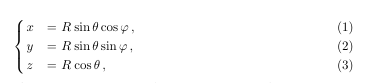
On doing cases in displayed math, one can use \begin{cases}...\end{cases},
but the numbering for such a command is one time for the entire case
statement as in the following:
\begin{equation}
\begin{cases}
x &= R \thin \sin \theta \cos \varphi\,,\\
y &= R \thin \sin \theta \sin \varphi\,,\\
z &= R \thin \cos \theta\,,
\end{cases}
\end{equation}
to produce:
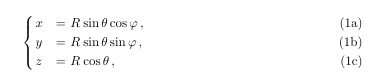
If, however, you want to have each line given a line number, you can use
the cases package, begining with the statement:
\usepackage{cases}
in the preamble (heading) of the document.
\begin{numcases}{}
x &= $R \thin \sin \theta \cos \varphi$\,,\\
y &= $R \thin \sin \theta \sin \varphi$\,,\\
z &= $R \thin \cos \theta$\,,
\end{numcases}
will produce:
\begin{subnumcases}{}
x &= $R \thin \sin \theta \cos \varphi$\,,\\
y &= $R \thin \sin \theta \sin \varphi$\,,\\
z &= $R \thin \cos \theta$\,,
\end{subnumcases}
will produce the following 'subnumbering' output:
Next,
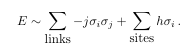
The code to this is:
\begin{equation}
\doubleobsigma = \tanh [- 2dJ\obsigma + h] \beta \,.
\end{equation}
which uses the macro
\newcommand{\doubleobsigma}{\rlap{$\sigma$}\kern1.2pt\overline{\overline{\phantom{\fiverm I}}}\kern.4pt{}}
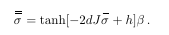
The code to this is:
\begin{equation}where \definedas comes from \newcommand{\definedas}{\equiv}.
E \sim \sum_{\mbox{links}} -j \sigma_i\sigma_j + \sum_{\mbox{sites}} h \sigma_i\,.\label{eq:Esim+Eternal.magenticfield}
\end{equation}
Next,
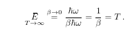
The code to this is:
\begin{equation}
\underset{T\to\infty}{\obE} \overset{\beta\to0}{=}
\frac{\hbar \omega}{\beta \hbar \omega} = \frac{1}{\beta} = T\,.
\end{equation}
The purpose of this graphic is to show the use of \underset and \overset commands.
Next,
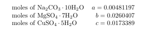
The code to this is:
\begin{tabular}{l r}
\text{moles of \ce{Na2CO3}\bdot 10\HTO} & $a = 0.00481197$\\
\text{moles of \ce{MgSO4}\bdot7\HTO}& $b = 0.0260407$\\
\text{moles of \ce{CuSO4}\bdot5\HTO}&$c = 0.0173389$
\end{tabular}
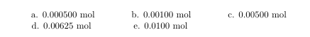
The code to this is:
$
\begin{matrix}
&\text{a. 0.000500 mol} &&&&\text{b. 0.00100 mol} &&&&\text{c. 0.00500 mol}\\
&\text{\!\!d. 0.00625 mol} &&&&\text{\!e. 0.0100 mol} &&&&
\end{matrix}
$
To set a tilde to the desired height when I want it to be an 'exponent,'
![]()
I use something like
(\rho^{1/2} e^{\smallhalf i\beta}R)^{\raisebox{2pt}{$\sim$}}where the \sim acts as the tilde and the \raisebox{2pt} allows me
Next, how to place a slash over a character, like this:
![]()
We could try the \cancel command, but that doesn't give us
the power to precisely place it. So, I'll show here what I did
by using some PlainTeX commands, which you can look up
if you wish:
\def\thin{\hskip.75pt{}}
\newlength{\gnat}
\settowidth{\gnat}{$\thin\slash$}
\newlength{\Gnat}
\settowidth{\Gnat}{$\,\slash$}
Then, the LaTeX code looks like:
\gamma^\nu\cdot\slash\hskip-\Gnat W_\nuIf you want to try the \cancel command, use the \usepackage{cancel}
By the way, I invented the command '\thin' to be able to quickly add
a little extra space between symbols in TeX math expressions that look
to me to be too close together. One that's built into LaTeX is '\,'.
In the above macros, I tried to use an automated approach to defining
the macro to slash a character (/), but it may be a lot easier just to set the
horizontal movement of the slash character by hand, so to speak. The
following are also possible for the letters a,b,c:
\def\slasha{\hbox{$ \slash\hskip-5.07pt a$}}
\def\slashb{\hbox{$ \slash\hskip-5.07pt b$}}
\def\slashc{\hbox{$ \slash\hskip-5.07pt c$}}
The \hbox{} creates its own environment, wherever it is. Then,
one defines the math environment within it. The default math style
created by one left and one right dollar sign is the textstyle. To get
the displaystyle, use the command '\displaystyle' right after the
left dollar sign. I didn't need to do that for these macros.
I wanted to use the symbol for empty set -- the one that uses the zero with the
slash through it. I didn't like thet one resident in LaTeX, so I made my own.
\font\elevenrm=cmr11The result is this:
\def\myemptyset{\mbox{\elevenrm0}\raisebox{0.5pt}{\kern-5.4pt/}}
I wanted to rescale a mathematical symbol arbitrarily large, but it turned out
that it only needed to be enlarged 1.2 times. The ability to do this resides in the
\scalebox command. The syntax is as this:
\scalebox{scaling factor}{thing to be rescaled}So, when I went to rescale the symbol for the 'unity' symbol, I used
\def\unity{\scalebox{1.2}{$\mathbb{1}$}}and then typed in '\unity'. The result is this:
I wanted to make my own symbol to represent an ideal of a ring. I chose
to the hollow-tipped left-pointing arrow. So, I had to construct it, and
it wasn't hard. I used this
$\triangleleft\hskip-5pt-$which looks like this:
There is always something new to learn when typesetting mathematics in LaTeX.
How should we typeset the following:  ? I used this:
\lim_{\overset{\scalebox{0.75}{$t\to +\infty$}}{t'\to-\infty}}To use the \overset command, one thing is placed over another thing, but in this case