My importing of graphics into a LaTeX has been as of late limited to three formats: PNG, JPEG, Xy-Pic,
and PicTex. I found that LaTeX will also take PDF format, which is useful for vector graphics (though I
haven't used this format myself). There are probably other supported formats, as well, but this is just
a barebones introduction to the subject, so I'll keep this article brief.
Go to the following link to view my write up on Xy-pic graphics program, which is used to produce nice-looking
line graphics such as flow charts, block diagrams, and commutative diragrams (for category theory) and similar
mathematical flow diagrams, of which I'll demonstrate a few.
Click this link for Xy-pic graphics program.
By the way, PicTeX is a really old format, but it seems that it is still supported. I'll get to that format
at the end.
Just a note about EPS format. Recently, I found a bunch of EPS files that I was using for a math paper,
but they didn't work anymore. I don't know why. If this happens to you, you might happen to have a utility
to convert one graphic format to another, but if you don't, there are free utilities on the Web that you can
upload your graphics files to and they will convert the graphic to the format you request and then you just
down load them at that point. That's what I did to convert the EPS files to PNG format, and it worked fine.
But I also have occasion to convert to SVG format so I can import them into a graphics program to edit them
as I please.
Is one graphics format better than the others? Well, probably. I presume that the more recent formats
are generally better than the earlier formats.
Now we see some LaTeX code for the following graphic:
The following is the LaTeX code for the figure above:
\vskip.1inSo, there are two distinct things to go over at this point:
\centerline{\includegraphics[height=1.552in]{BisectorsCon.png}}
\vskip.1in
\begin{quote}
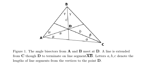
\text{\ninerm\hskip.5in Figure 1. The angle bisectors from $\bA$ and $\bB$ meet at $\bD$. A line is extended}\newline
\text{\ninerm\hskip.5in from $\bC$ though $\bD$ to terminate on line segment$\overline{\bA\bB}$. Letters $a,b,c$ denote the}\newline
\text{\ninerm\hskip.5in lengths of line segments from the vertices to the point $\bD$.}
\end{quote}
How to import the graphic, size it the way you want, and then
make a caption for it:
First, this is LaTeX, so I'm sure there are a lot of other ways to do this besides the way I do it. I use
the graphics import command \includegraphics, which requires the package \usepackage{graphicx}.
So, you can start off with this command and try others as well at some point. The graphics file name I used
here is 'BisectorsCon.png'. I made this file myself in a graphics program, and we'll go over that later.
As for the height, how does one know what number to use for it? Well, just try something and adjust it
either to your personal preferences or to the constraints imposed by whatever publishing entity you are
working with, or both.
Where should I place the graphics file to be scene by the LaTeX program? Simple. Put it in the same folder
that you have the LaTeX file. Thjere are other ways to do this by using the PATH command, but since this is
just an introduction to LaTeX, I will not go over it or even recommend it.
There are caption commands in LaTeX. I tried them long ago but decided that I'll use what amounts
to Plain TeX commands. Why? Because I found that I had problems with the right justification of the
text in the shorter-width column of the caption. LaTeX is great for right justification under normal
conditions, meaning that the width is standard. But when the width becomes narrow, it can break down.
That means that you can have big gaps between words. So, I decided that I'll leave the captions right-ragged
and use primitive commands. Yes, it involves more time and effort, but I retain the formatting control I want.
I've used Illustrator before and nothing else I've used can compare to it --- but....If you look through
the graphics I use for my math papers, they're mostly composed of sticks and circles, or maybe an
occasional bezier curve. Adobe Illustrator is designed for high-end users, and for them it's worth it.
But I'm not going to pay the price for that program when I know I will be using only 2% of its capability.
So, I opt for Inkscape. The normal Inkscape file is an SVG file format and then you export the type of
graphic you want from it. I usually export them as PNG files, which is how I produced the graphic above.
Now, regardless of the graphics program you use, you have to take the time to learn how it works.
There are usually YouTube videos and websites for help. Sometimes graphics are indispensable, and even
when they're not, they can still be highly useful. One of the most common gripes I remember from reviews
of some high-end math books is that they don't contain enough graphics.
Okay, to take some of the pain out of making graphics, plan on reusing the ones you've already made.
This is what I do: Once I make an SVG file, I make a COPY of it, together with a PNG version of it,
and save them to a central collection folder. Then I turn on the file viewing feature so that it displays
pictures of the files. Now, Windows won't render an image of the SVG file, but it will render an image of
the corresponding PNG file. Then, when you go to make a brand new graphic, you look at the graphics in
your central folder for a graphic that's as close to what you need as you can get, and then COPY that SVG
file to another folder and rename it and then merely edit it. When you have it in the final state you want,
make a COPY of that file (with its PNG file version) to the central folder for future use.
If I have two graphics that I want to put side-by-side in LaTeX, rather than one atop the other, I have
two ways to do this. The easiest may be to combine the two separate graphics into a single graphic.
The other way is to use PlainTeX commands to accomplish the same thing. For my example, I have
two simple graphics, neither of which will take up much width on the page, and to simply place them
one on top of the other looks silly. So I set them on the "same line" by some simple PlainTeX commands.
Each graphic has both image and subtext. Therefore, I need to put each graphic into its own \vbox.
But if that's all I do, they will still stack up vertically. To force them to display themselves
side-by-side, I place them both inside an \hbox:
\hbox{
\vbox{\hskip.45in\includegraphics[height=1.0271in]{Proton-Decay-muon+.png}
\vskip.151in
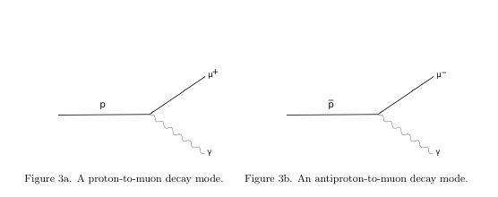
\no \text{\ninerm\hskip.25in Figure 3a. A proton-to-muon decay mode.}}
\vbox{\hskip-2.8485in\includegraphics[height=1.0271in]{Proton-Decay-muon-.png}
\vskip.151in
\no \text{\ninerm\hskip-3.1485in Figure 3b. An antiproton-to-muon decay mode.}
}
}
Warning: I suppose that someone has long ago invented a more LaTeXish way of doing this.
Even so, if you're not afraid of tweeking the numerical values, you have a lot of control
with this method.
To use PicTeX, you need the file 'PicTeX.tex' which you can download from
https://www.ctan.org/tex-archive/graphics/pictex/
Feel free to use any of the following PicTeX code. And, no doubt, to code can be improved.
I keep a copy of this file in the folder my TeX files are in that use it. I used the
following PicTeX code to produce the graphic after it:
$$\vbox{
\setcoordinatesystem units <.75in,.75in>
\beginpicture
\linethickness=.5pt
\setquadratic \plot 1.1 1.8 0.5 2.5 1.4 2.5 /
\put {$\bx(s)$} at 0.3 2.56
\put {$\bT(s)$} at 1.2 2.9
\put {$\bT(s+\Delta s)$} at 1.85 2.6
\put {$\bullet$} at 0.55 2.55
\put {$\bullet$} at 0.85 2.6
\arrow <.12in> [.2,.67] from 0.55 2.55 to 1.0 2.8
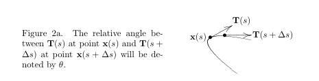
\arrow <.12in> [.2,.67] from 0.85 2.6 to 1.4 2.6\put {\vbox{\hsize=2.2in\no{}Figure 2a. The relative angle between $\bT(s)$ at
point $\bx(s)$ and $\bT(s+\Delta s)$ at point $\bx(s+\Delta s)$ will be denoted by
$\theta$.}} at -1.9 2.3
\endpicture
}$$
I used the following PicTeX code to produce the graphic after it (You can ignore the lines that have a % sign on them.):
$$\vbox{
\setcoordinatesystem units <.75in,.75in>
\beginpicture
\linethickness=.5pt
% \setquadratic \plot 3.5 1.5 3.0 2.1 2.5 2.2 /
% \setquadratic \plot 3.0 1.5 2.8 1.9 2.5 2.0 /
% \setquadratic \plot 2.3 2.1 2.5 2.2 2.7 2.4 /
% \setquadratic \plot 2.3 2.1 2.5 2.0 2.7 1.7 /
% \setquadratic \plot 2.0 1.0 1.8 0.90 1.6 0.70 /
% \setquadratic \plot 2.0 1.0 1.8 1.10 1.6 1.30 /
\setquadratic \plot 0.5 2.0 0.9 1.3 1.8 0.9 /
\setquadratic \plot 1.8 0.9 2.9 0.8 3.4 1.1 /
\setquadratic \plot 3.4 1.1 3.4 1.5 3.1 1.8 /
\setquadratic \plot 3.1 1.8 2.5 2.5 3.4 2.5 /
% \ninepoint
\put {$\bx(s)$} at 2.3 2.56
\put {$\bT(s)$} at 3.2 2.9
\put {$\bN(s)$} at 3.3 2.3
\put {$-\bB(s)$} at 2.2 3.0
\put {$\cal C$} at 0.9 1.7
\put {$\bullet$} at 2.55 2.55
\arrow <.12in> [.2,.67] from 2.55 2.55 to 3.0 2.8
\arrow <.12in> [.2,.67] from 2.55 2.55 to 2.55 3.1
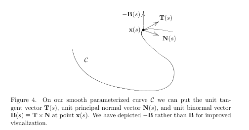
\arrow <.12in> [.2,.67] from 2.55 2.55 to 3.0 2.4\put {\vbox{\no{}Figure 4. On our smooth parameterized curve $\cal C$ we can put
the unit tangent vector $\bT(s)$, unit principal normal vector $\bN(s)$, and unit
binormal vector $\bB(s)\equiv \bT\cross\bN$ at point $\bx(s)$. We have depicted
$-\bB$ rather than $\bB$ for improved visualization. }} at 1.9 .2
\endpicture
}$$
I used the following PicTeX code to produce the graphic after it:
$$\vbox{
\setcoordinatesystem units <.75in,.75in>
\beginpicture
\linethickness=.5pt
\put {\vrule height .4pt width 280pt} at 2.4 -.3
\put {\vrule height 150pt width .4pt} at 1.9 0.3
\put {$ct$} at 2.1 1.35
\put {{\bf x}} at 4.65 -.15
\put {timeline for frontend of rod} at 3.5 -.63
\put {timeline for rearend of rod} at .4 0.8
\setlinear \plot 1.3 -1.2 1.8 1.8 /
\plot 2.2 -1.2 2.7 1.8 /
\linethickness=5.5pt
\plot 1.45 -.285 2.43 0.07 /
\linethickness=.5pt
\setdashes \setlinear \plot 1 -.48 3 .3 /
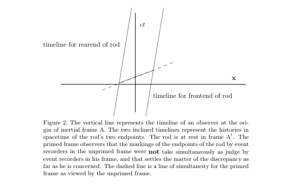
\put{\vbox{\hsize=4.3in\baselineskip=11pt\ninerm\noindent{}Figure 2.\ The
vertical line represents the timeline of an observer at the origin of inertial
frame A. The two inclined timelines represent the histories in spacetime of the
rod's two endpoints. The rod is at rest in frame A$'$. The primed frame
observers that the markings of the endpoints of the rod by event recorders
in the unprimed frame were {\bf not} take simultaneously as judge by event
recorders in his frame, and that settles the matter of the discrepancy as far as
he is concerned. The dashed line is a line of simultaneity for the primed frame
as viewed by the unprimed frame.}} at 2.2 -2.1
\endpicture
}$$
I used the following PicTeX code to produce the graphic after it:
$$\vbox{
\setcoordinatesystem units <.75in,.75in>
\beginpicture
\linethickness=.5pt\circulararc 360 degrees from 2 .1 center at 2 .4
\circulararc 360 degrees from 1.6 -.3 center at 1.6 -.6\putrectangle corners at -.5 2.5 and 4.5 0
\dimen0=.375in
\setplotarea x from -.5 to .5, y from -.5 to .5
\dimen2=6.28319\dimen0 \divide\dimen2 by 5
\setdashpattern <.2\dimen2, .2\dimen2, .2\dimen2, .2\dimen2>
\circulararc 360 degrees from 2 -.3 center at 2 -.6\setdots
\putrule from 1.98 .7 to 1.98 2.5
\setsolid
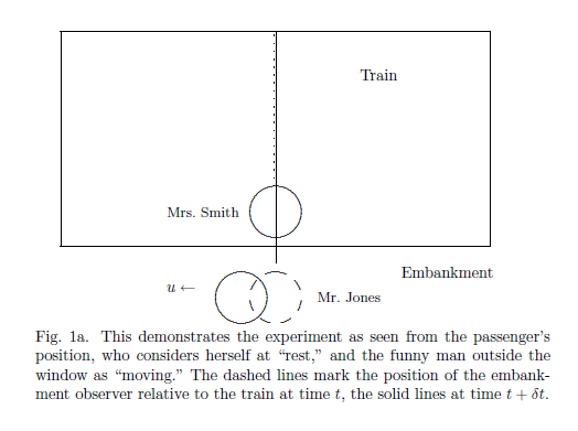
\putrule from 2.01 2.5 to 2.01 -.2\put {\vbox{\hsize=4.5in\noindent{}Fig.\ 1a. This demonstrates the
experiment as seen from the passenger's position, who considers herself at
``rest," and the funny man outside the window as ``moving." The dashed lines
mark the position of the embankment observer relative to the train at time
$t$, the solid lines at time $t+\delta{}t$.}} at 2.2 -1.4
\put {\ninepoint Mr.\ Jones} at 2.7 -.6
\put {\ninepoint Mrs.\ Smith} at 1 .4
\put {Train} at 3.2 2
\put {Embankment} at 4 -.3
\put {$u \leftarrow$} at .9 -.5
\endpicture
}$$
I used the following PicTeX code to produce the graphic after it:
$$\vbox{
\setcoordinatesystem units <.75in,.75in>
\beginpicture
\linethickness=.5pt
\put {\vrule height .4pt width 280pt} at 2.4 0
\put {\vrule height 150pt width .4pt} at 1.9 0
\put {$ct$} at 1.7 1.35
\put {$ct'$} at 3.1 1.35
\put {${\bf x}(t>0)$} at 4.65 -.15
\setlinear \plot 2.5 -1.4 2.95 1.45 /
\setquadratic \plot 2.4 0.0 2.5 0.2 2.6 0.5 /
\setquadratic \plot 2.6 0.5 2.63 0.7 2.6 0.8 /
\setquadratic \plot 2.6 0.8 2.65 1.0 2.7 1.2 /
\setquadratic \plot 2.4 0.0 2.35 -0.34 2.4 -.5 /
\setquadratic \plot 2.4 -0.5 2.45 -0.6 2.4 -0.8 /
\setquadratic \plot 2.4 -0.8 2.2 -1.1 2.1 -1.4 /
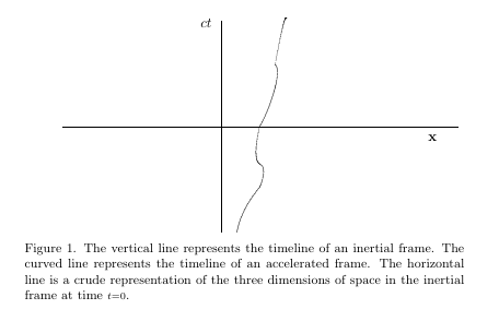
\put{\vbox{\hsize=4.3in\baselineskip=11pt\ninerm\noindent{}Figure 2. This figure
is a slight modification of Fig.\ 1. The $ct'$ timeline of the primed inertial
frame has been added. For the purpose of extended relativity, all three
timelike curves represent reference frames.}} at 2.2 -1.9
\endpicture
}$$
$$\vbox{
\setcoordinatesystem units <.75in,.75in>
\beginpicture
\linethickness=.5pt
\putrectangle corners at 2.0 5.0 and 3.5 4.5\putrectangle corners at 0.0 4.0 and 1.5 3.5
\putrectangle corners at 4.0 4.0 and 5.5 3.5\putrectangle corners at -1.0 3.0 and 0.5 2.5
\putrectangle corners at 1.0 3.0 and 2.5 2.5
\putrectangle corners at 2.75 3.0 and 4.8 2.25
\putrectangle corners at 5.0 3.0 and 6.25 2.25\putrectangle corners at 0.0 2.25 and 1.5 1.75
\putrule from 2.0 4.75 to .75 4.75
\putrule from 3.5 4.75 to 4.75 4.75
\putrule from .75 4.75 to .75 4.0
\putrule from 4.75 4.75 to 4.75 4.0
\put {$\downarrow$} at .75 4.1
\put {$\downarrow$} at 4.75 4.1\putrule from 0.0 3.75 to -.25 3.75 %across
\putrule from 1.5 3.75 to 1.75 3.75 %across
\putrule from 4.0 3.75 to 3.75 3.75 %across
\putrule from 5.5 3.75 to 5.625 3.75 %across
\putrule from -.25 3.75 to -.25 3.0 %down
\putrule from 1.75 3.75 to 1.75 3.0 %down
\putrule from 3.75 3.75 to 3.75 3.0 %down
\putrule from 5.625 3.75 to 5.625 3.0 %down
\putrule from .75 3.5 to .75 2.25 %down, fourth level
\put {$\downarrow$} at -.25 3.1
\put {$\downarrow$} at 1.75 3.1
\put {$\downarrow$} at 3.75 3.1
\put {$\downarrow$} at 5.625 3.1
\put {$\downarrow$} at .75 4.1
\put {$\downarrow$} at .75 2.35\ninepoint
\put {arche-definition} at 2.45 4.75
\put {quasi-definition} at .45 3.75
\put {``true" definition} at 4.45 3.75
\put {replacement} at -.6 2.75
\put {implicit} at 1.5 2.75
\put {extensional, intensional} at 3.5 2.75
\put {ostensional, impredicative} at 3.5 2.50
\put {lexical} at 5.4 2.5
\put {stipulative} at 5.4 2.75
\put {operational} at .5 2.0
%
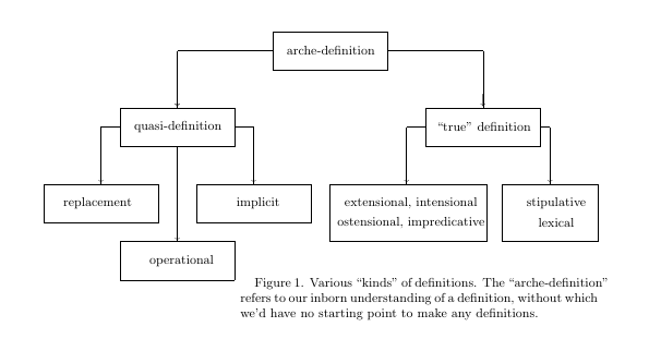
\put {\vbox{\hsize=3.5in{}Figure 1. Various ``kinds" of definitions. The
``arche-definition" refers to our inborn understanding of a definition, without
which we'd have no starting point to make any definitions.}} at 3.6 1.5
\endpicture
}$$
$$\vbox{
\setcoordinatesystem units <.75in,.75in>
\beginpicture
\linethickness=.5pt
\putrectangle corners at 2 1.5 and 4.4 .5
\putrectangle corners at 0 2.5 and 5 0
\setquadratic \plot 3.5 1.5 3.0 2.1 2.5 2.2 /
\setquadratic \plot 3.0 1.5 2.8 1.9 2.5 2.0 /\setquadratic \plot 2.3 2.1 2.5 2.2 2.7 2.4 /
\setquadratic \plot 2.3 2.1 2.5 2.0 2.7 1.7 /\setquadratic \plot 2.0 1.0 1.8 0.90 1.6 0.70 /
\setquadratic \plot 2.0 1.0 1.8 1.10 1.6 1.30 /\setquadratic \plot 0.5 2.0 0.9 1.3 1.8 0.9 /
\setquadratic \plot 1.0 2.0 1.3 1.4 1.8 1.1 /\ninepoint
\put {{\titlefont Predicate logic}} at .9 2.2
\put {{\titlefont Sentential logic}} at 2.8 1.0
\put {de-quantified} at 0.3 1.0
\put {sentences in} at 0.5 0.8
\put {re-quantified} at 3.5 2.0
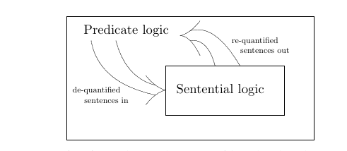
\put {sentences out} at 3.7 1.8\put {\vbox{\no{}Figure 4. Before inference rules are used on sentences of the
Predicate logic, they are first reduced to simple unquantified sentences of
Sentential logic, then generalized back into the quantified predicate
sentences.}} at 1.9 -.5
\endpicture
}$$
$$\vbox{
\setcoordinatesystem units <.75in,.75in>
\beginpicture
\linethickness=.5pt
\circulararc 360 degrees from 3.75 1.0 center at 3.75 .3
\put {\vrule height .4pt width 200pt} at 3.0 -1
\put {\vrule height 150pt width .4pt} at 1.9 0
\put {$y$} at 1.7 1.3
\put {$x$} at 4.65 -1.15
\put {$\bullet$} at 3.75 .3
\arrow <.12in> [.2,.67] from 3.75 .3 to 3.2 .7
\put {$a$} at 3.85 0.35
\put {$r$} at 3.4 0.45
%\put {$b$} at 4.15 0.65
%\put {$\bullet$} at 4.2 0.5
\put {$\Gamma$} at 4.25 1.0
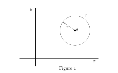
\put {Figure 1} at 3.4 -1.5
\endpicture
}$$
\hskip.1in\hbox{
\setcoordinatesystem units <.75in,.75in>
\beginpicture
\linethickness=.5pt
\putrectangle corners at 2 1.5 and 4.4 .25
\putrectangle corners at 0 2.5 and 5 0
\setquadratic \plot 2.0 1.0 1.8 0.90 1.6 0.70 /
\setquadratic \plot 2.0 1.0 1.8 1.10 1.6 1.30 /\setquadratic \plot 0.5 2.0 0.9 1.3 1.8 0.9 /
\setquadratic \plot 1.0 2.0 1.3 1.4 1.8 1.1 /\ninepoint
\put {{\bigfont water $\Delta W$}} at .4 2.2
\put {{\titlefont System (before):}} at 2.8 1.2
\put {{\bigfont radiator fluid}} at 2.8 0.8
\put {{\bigfont $W_1\oplus{}A_1$}} at 2.8 0.5
\put {added in} at 0.3 1.0
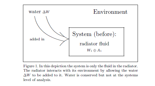
\put {{\titlefont Environment}} at 3.5 2.2\put {\vbox{\hsize=3.75in\no{}Figure 1.\ In this depiction the system is only
the fluid in the radiator. The radiator interacts with its environment by
allowing the water $\Delta{}W$ to be added to it. Water is conserved but not at
the systems level of analysis.}} at 2.2 -.5
\endpicture
}
\hskip.25in\hbox{
\setcoordinatesystem units <.75in,.75in>
\linethickness=.5pt
\putrectangle corners at 1 1.8 and 4.4 .3
\putrectangle corners at 0 2.5 and 5 0
\putrule from 1 1.4 to 4.4 1.4
% \putrule from 1 1.0 to 4.4 1.0
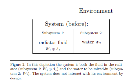
\putrule from 2.8 0.3 to 2.8 1.4\ninepoint \put {{\titlefont System (before):}} at 2.2 1.6
\put {{\titlefont Environment}} at 3.5 2.2
\put {Subsystem 1:} at 1.6 1.2
\put {Subsystem 2:} at 3.3 1.2
\put {{\bigfont radiator fluid}} at 1.6 0.8
\put {{\bigfont $W_1\oplus{}A_1$}} at 1.6 0.5
\put {{\bigfont water $W_2$}} at 3.3 0.8\put {\vbox{\hsize=3.75in\no{}Figure 2. In this depiction the system is both the
fluid in the radiator (subsystem 1: $W_1\oplus{}A_1$) and the water to be
mixed-in (subsystem 2: $W_2$). The system does not interact with its environment by
design.}} at 2.2 -.5
}
$$\vbox{
\setcoordinatesystem units <10pt,10pt>
\beginpicture
\linethickness=.3pt
\setdashes
% horizontal
\putrule from -4.7 6 to 4.5 6
\putrule from -5.7 1 to 4.5 1
% vertical
\putrule from -8 5 to -8 2
\putrule from 8 5 to 8 2
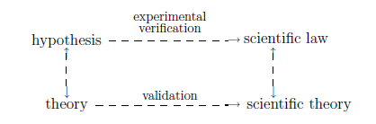
\put {\twelverm hypothesis} at -8 6
\put {\twelverm scientific law} at 9 6.2
\put {\twelverm theory} at -8 1
\put {\twelverm scientific theory} at 10 1
\put {experimental} at 0 7.8
\put {verification} at 0 7.0
\put {validation} at 0 1.8
\put {$\rightarrow$} at 5 5.97
\put {$\rightarrow$} at 5 0.962
\put {$\uparrow$} at -7.99 5
\put {$\uparrow$} at 8 5
\put {$\downarrow$} at -7.98 2
\put {$\downarrow$} at 8.025 2
\endpicture
}$$
$$\vbox{
\setcoordinatesystem units <.75in,.75in>
\beginpicture
\linethickness=.5pt
\putrectangle corners at 2 1.5 and 4.4 .5
\putrectangle corners at 1.5 2 and 4.7 .25
\putrectangle corners at 0 2.5 and 5 0
\ninepoint
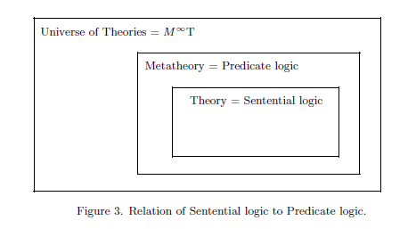
\put {Universe of Theories = $M^\infty$T} at .9 2.3
\put {Metatheory = Predicate logic} at 2.4 1.8
\put {Theory = Sentential logic} at 2.9 1.3
\put {Figure 3. Relation of Sentential logic to Predicate logic.} at 2.4 -.3
\endpicture
}$$